Truth and Integrity in State Budgeting - Preventing the Next Fiscal Crisis

Foreword
This report marks the Volcker Alliance’s second annual assessment of US state budget practices. Covering the fiscal years 2016, 2017, and 2018, the study grades states’ success in pursuing transparent and fiscally sustainable procedures as they estimate their revenues and expenditures and attempt to keep them in balance not only at the start of the fiscal year but as it progresses.
Because the US federal system is composed of fifty sovereign states, it is essential to assess and compare the quality of their budget practices against a common set of standards. As we did in the 2017 report, we gave states grades of A to D-minus, the lowest possible mark, for their practices in five areas that are the building blocks of budgeting nationwide:
- budget forecasting, in which we evaluate how and whether states estimate revenues and expenditures for the coming fiscal year and the long term;
- budget maneuvers, in which we gauge dependence on one-time actions to offset recurring expenditures;
- legacy costs, in which we assess how well states are funding promises made to public employees to cover retirement costs, including pensions and retiree health care;
- reserve funds, in which we examine the condition of general fund reserves as well as rainy day funds and rules governing their use and replenishment; and
- budget transparency, in which we scrutinize disclosure of budget information, including debts, tax expenditures, and the estimated cost of deferred infrastructure maintenance.
In this report, we also compared states’ budgetary grades to marks given the year before and offer best practices in each of the five budget categories.
Introduction
More than nine years after the end of the deepest US recession since the 1930s, states are finally reaping the fruits of the recovery, with thirty-four reporting that revenues had rebounded to pre-recession levels after adjusting for inflation. Even amid the economic boom, though, many states still struggle to balance budgets in the face of mounting obligations for health care, infrastructure, education, and public employee retirement costs. While some progress has been made since our publication in 2017 of Truth and Integrity in State Budgeting: What Is the Reality?, these fiscal challenges continue to vex policymakers and taxpayers alike.
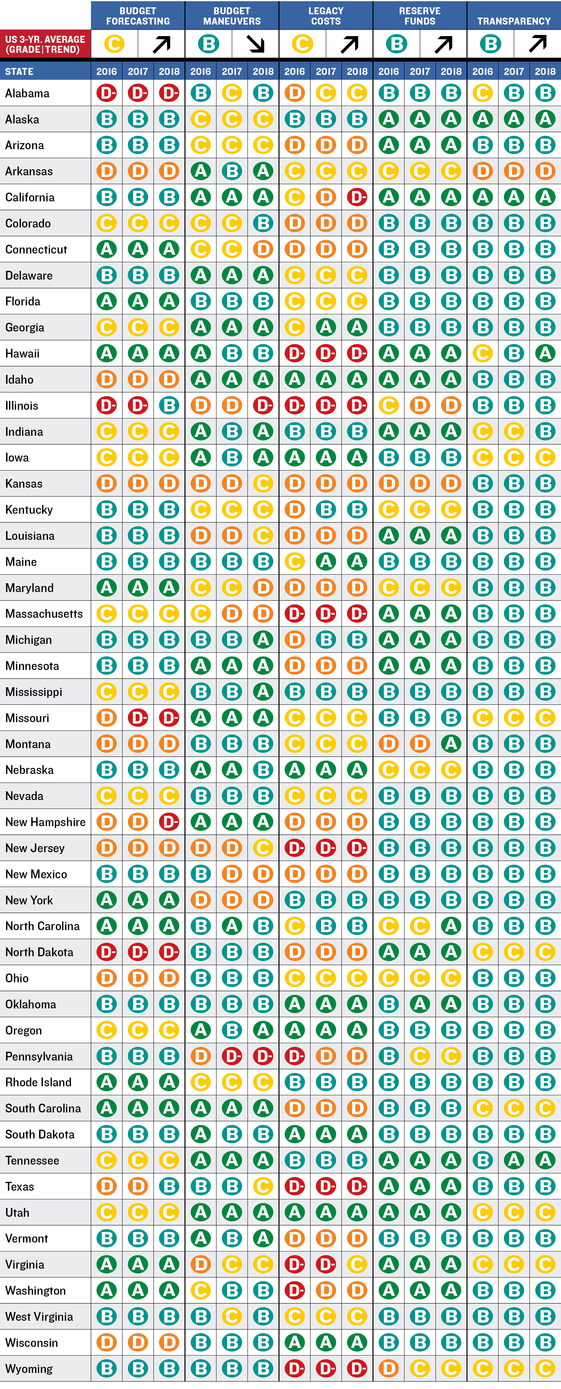
Forty-nine states require balanced budgets by law; Vermont follows the example of its peers by tradition. Yet scrutiny of budgetary practices is vital, because states can achieve balance in various ways—some more desirable than others. As we did in 2017, we have graded states in five areas critical to their ability to maintain balanced and sustainable budgets. We ranked states on a scale of A to D-minus. (There is no F grade—even the most fiscally challenged states have some good budget practices.) The grading period for this report spans fiscal 2016, 2017, and 2018, and evaluates these areas:
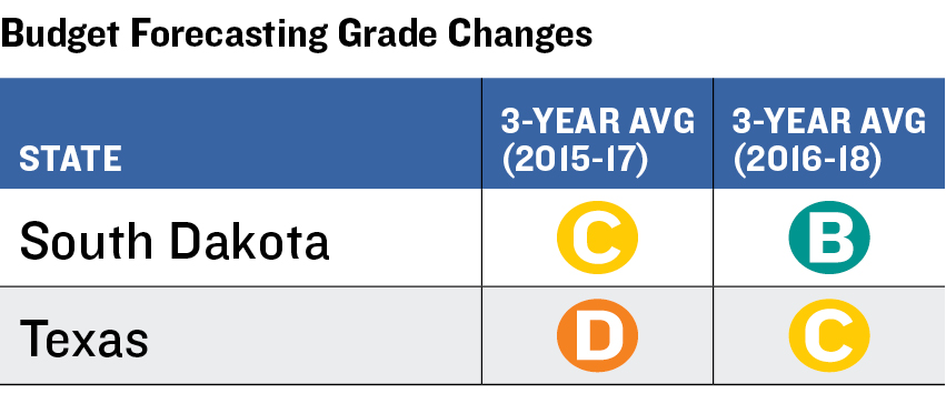
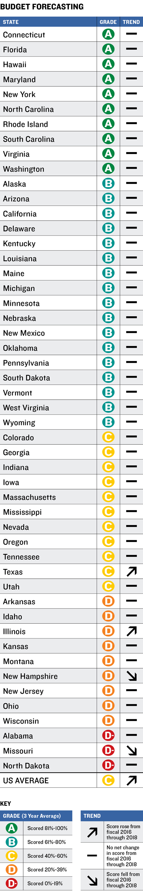
- Budget forecasting—how and whether states estimate revenues and expenditures for the coming fiscal year and the long term. For fiscal 2016 through 2018, three-year average grades in this category increased from the previous year for two states and were unchanged for forty-eight.
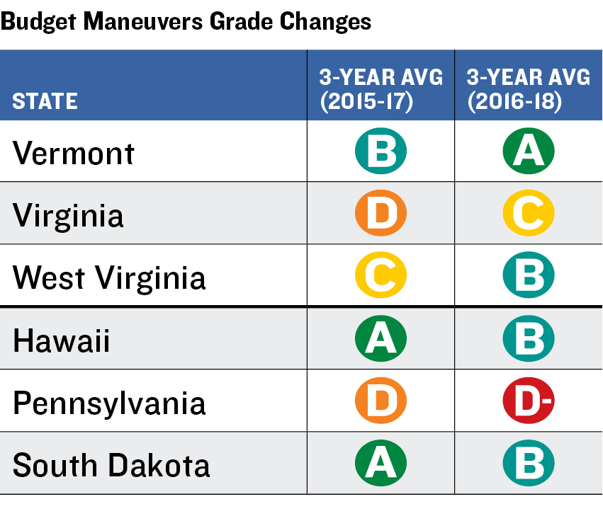
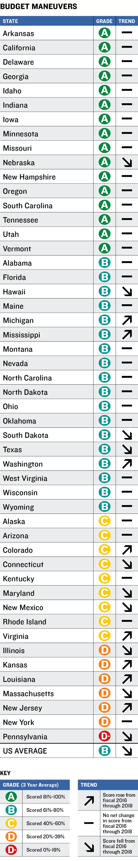
- Budget maneuvers—primarily how much states depend on one-time actions to offset recurring expenditures. Three-year average grades increased for three states, declined for three, and were unchanged for forty-four.
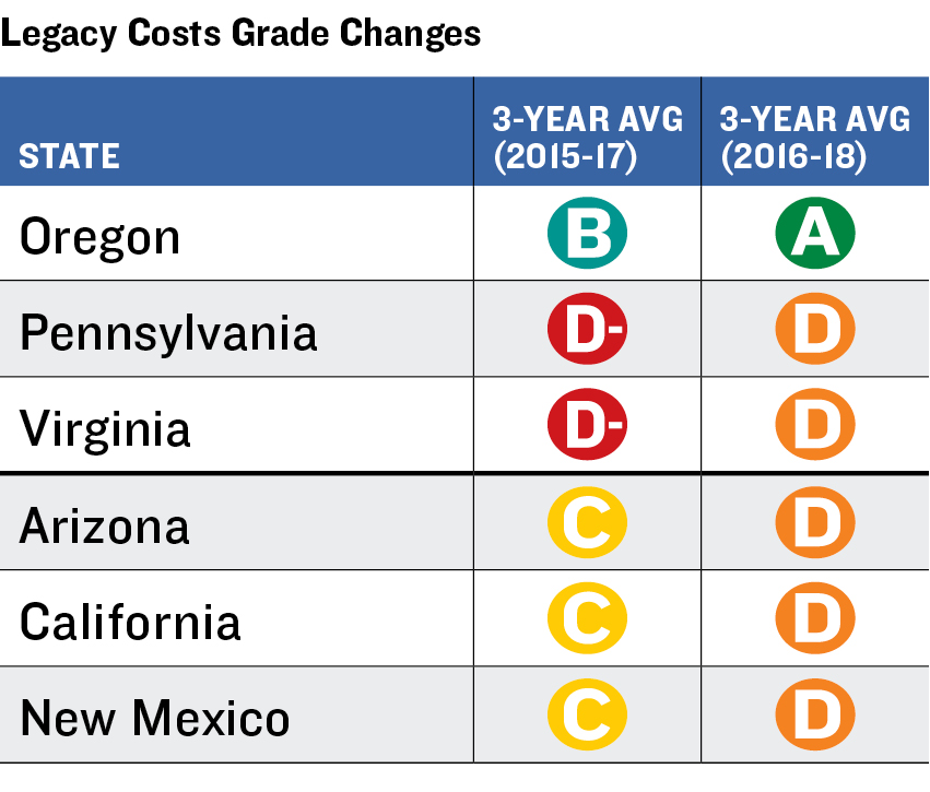
- Legacy costs—how well states are funding promises made to public employees to cover retirement costs, including pensions and retiree health care. Three-year average grades increased for three states, declined for three, and were unchanged for forty-four.
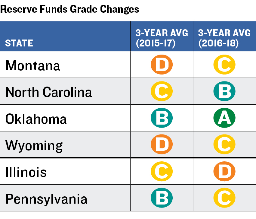
- Reserve funds—both the health of general fund reserves and rainy day funds and whether governments have clear rules governing their use, replenishment, and relationship to historic revenue volatility. Three-year average grades increased for four states, declined for two, and were unchanged for forty-four.
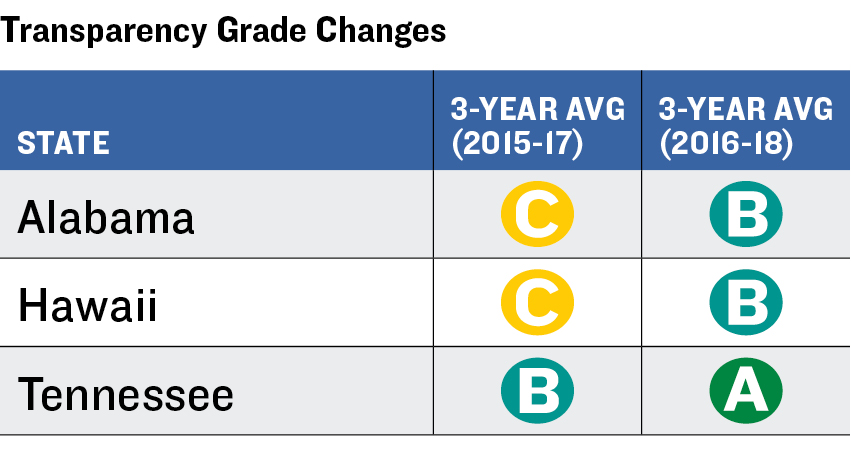
- Budget transparency—how completely states are disclosing budget information, including debts, tax expenditures, and the estimated cost of deferred infrastructure maintenance. Three-year average grades increased for three states and were unchanged for forty-seven.
State fiscal sustainability is of no small concern to the US economy or the federal government. As Volcker Alliance Chairman Paul A. Volcker stated in 2017, “The purposes and manner in which public funds are spent are matters basic to our well-being as a nation.” Indeed, states generate $2.1 trillion in annual revenue, equivalent to 10.3 percent of the nation’s gross domestic product. State and local governments—the latter heavily dependent on state budget funding—employ almost twenty million people.
Wide variations in population and tax and funding practices make it difficult to compare one state’s budget numbers against another. That is why we have chosen to focus on well-accepted best practices in the five key categories. The grades in this study are less an effort to fault states with low marks than one to prompt them to adopt policies that have been successfully used by others and can be applied nationwide.
This year’s three-year average grades in each overall category are unchanged from those in our 2017 report. (We have adjusted the 2017 grades for revisions in our research methodology; see Appendix C for an explanation.) And as was the case in 2017, the latest grades show that meeting promised public employee pension and other retirement costs remains perhaps the most formidable challenge facing many states. Six states received the lowest possible average grade of D-minus in legacy costs, and over twice as many scored only a D. Just eight states were awarded the top grade of A in the category. South Dakota was the single state with an overfunded pension plan, meaning it maintains a cushion that protects its ability to pay for scheduled retirement benefits. The only other state with a 100 percent funded pension was Wisconsin.
In total, states have accrued $1.35 trillion in unfunded public worker pension liabilities and $692 billion in unfunded obligations for other postemployment benefits (OPEB), largely retiree health care. With retirement costs restricting spending in other areas, it is probably not a coincidence that a number of states with D or D-minus in legacy costs—Illinois, Massachusetts, New Jersey, and Pennsylvania, for example—were also among those receiving a D or D-minus for budget-balancing maneuvers.
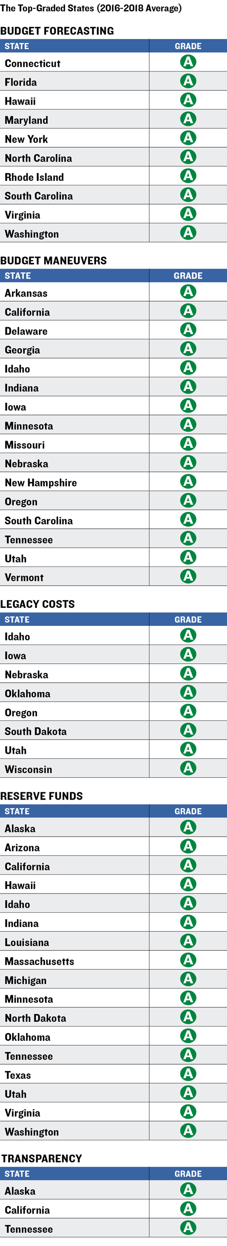
Grades for budget forecasting also indicate that states have considerable room for improvement, with twenty-three receiving grades of C or lower and only ten awarded As. Seventeen states received an A for reserves, a likely result of economic recovery. But only three were given the top grade for budgetary transparency, with common deficiencies being incomplete or nonexistent disclosure of deferred infrastructure maintenance and tax expenditure costs.
The grades and findings in this report are based on publicly available state budget documents and financial reports. Research for the study was conducted by teams of public finance professors and graduate students at City University of New York; Florida International University; Georgia State University; University of California, Berkeley; University of Kentucky; the Chicago and Springfield campuses of University of Illinois; and University of Utah. The schools’ efforts were augmented by Volcker Alliance staff, data consultants at the research firm Municipal Market Analytics, and special project consultants Katherine Barrett and Richard Greene.
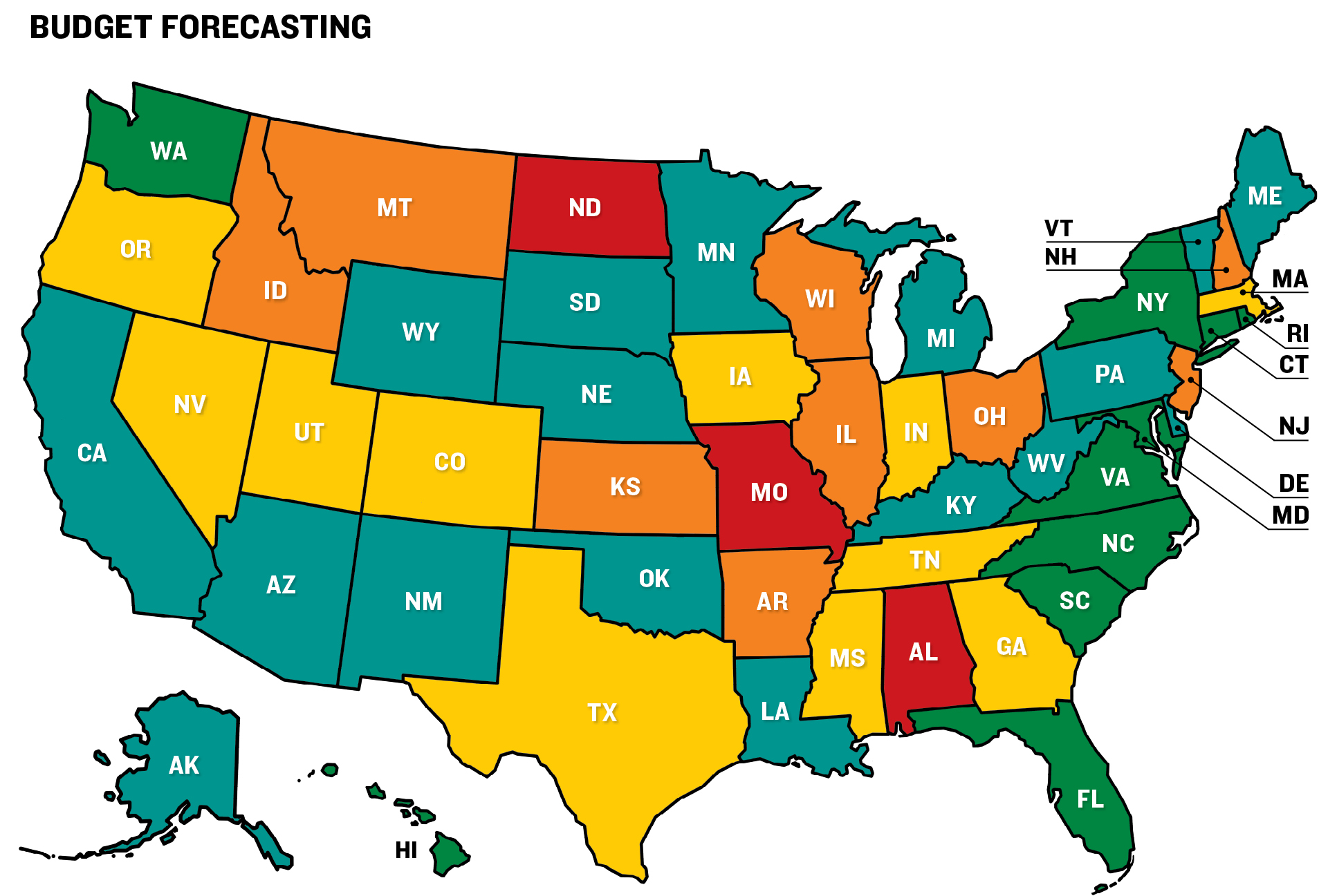
Grades awarded to states this year did not follow geographic patterns, and larger and smaller states were equally likely to score well or badly. Of the five smallest states by population, Alaska won an average A in transparency, South Dakota and Vermont received Bs, and North Dakota and Wyoming posted Cs. Grades also varied across categories within individual states. Hawaii, for example, received a D-minus in the legacy costs category, which covers pensions and other postemployment benefits, while earning an A for its work in budget forecasting.
The prolonged economic recovery that has followed the steep US recession has given states additional resources to pursue best practices. But the fiscal pressures felt keenly in the immediate wake of the last recession have not disappeared. To mitigate the impact of an economic downturn and help ward off budgetary crises, states should create more sustainable policies in flush times rather than wait until the next downturn forces them to struggle to stay afloat.
Conclusions
While forty-nine of the fifty states mandate balanced budgets, that does not mean their budgeting always follows best practices. Nor does it mean that a budget will remain balanced from enactment through the entire fiscal year or that officials fully disclose the techniques used to eliminate any shortfalls.
Many of the best practices cited in this report might be followed automatically if states were to adopt an accrual-style form of accounting instead of cash-based methods. Cash-based accounting, widely used by state governments, allows expenditures to be recognized only when bills are paid. This permits a government to commit to significant spending in one year but not reflect that decision until future years, when the payments are actually made.
A technique called modified accrual accounting is already required by the Governmental Accounting Standards Board (GASB) for municipal financial statements, including comprehensive annual financial reports (CAFRs). The method is designed to recognize future costs when a financial commitment is established.
GASB sets the standards for the generally accepted accounting principles (GAAP) used by state and local governments. To be in conformity with GAAP, governments must follow the board’s standards, which require the use of the modified accrual basis of accounting in their CAFRs. Following its near-bankruptcy in 1975, New York City was also legally required to construct budgets using GAAP. In the forty-three years since adopting the method, the nation’s most populous city has avoided the fiscal crises that have beset many other municipalities and states.
Absent a transition to modified accrual accounting for budgets, the best practices enumerated in this report and reflected in state grades can help policymakers in their quest for sustainable and transparent fiscal policies.
Following are examples of states that rely on some of the best practices laid out in this report and its two predecessors, Truth and Integrity in State Budgeting: What Is the Reality? (2017) and Truth and Integrity in State Budgeting: Lessons from Three States (2015).
BUDGET FORECASTING
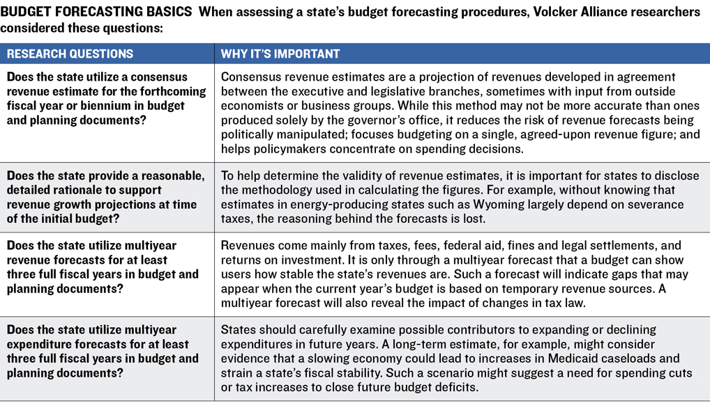
As we recommended in 2017, states should use a consensus approach to establish single, binding estimates for revenues and expenditures. In addition, for a budget to be of genuine help as a planning tool, it is important that it make predictions about revenues and expenditures for more than the following fiscal year. A one-year estimate does little to reveal structural deficits or built-in gaps between estimated revenues and anticipated expenditures that may return in budget after budget.
Utah is one state that has recently addressed this concern. Because of the absence of revenue or expenditure estimates beyond the current and upcoming fiscal year, it received a three-year average grade of C in budget forecasting for fiscal 2016 through 2018. But after the Volcker Alliance’s fiscal 2018 research cutoff date of October 31, 2017, the state improved its forecasting policies. A statute signed into law on March 19, 2018, obliges Utah’s Office of the Legislative Fiscal Analyst to produce a long-term budget every three years for programs appropriated from major funds and taxes. The law also requires the publication every three years, on a rotating basis, of analyses of revenue volatility and of stress tests of estimated revenue under various economic scenarios.
BUDGET MANEUVERS
States should pay for expenditures with recurring revenue earned in the same year. Yet forty states used at least one type of budget-balancing maneuver from 2016 to 2018 to cover shortfalls. The maneuvers often were repeated from year to year, a sign of a structural imbalance between revenues and spending.
Michigan has been weaning itself from budget maneuvers since 2015, when it received a C in this category. It scored Bs in the next two years and an A in 2018. The two areas in which it received no credit in 2015 were using revenue and cost shifting, and funding recurring expenditures with debt.
Thanks to an improving economy, Michigan was not pushed to use either practice in the fiscal year that ended September 30. With revenue outpacing estimates, both the Senate Fiscal Agency and the House Fiscal Agency projected a surplus of $278.5 million to $347.9 million in fiscal 2018, which minimized the need for budget maneuvers.
LEGACY COSTS
States should consistently make the contributions for pension and retiree health care plans that actuaries determine to be necessary. This presents a conundrum for states with severely underfunded pension systems. They need to maintain essential public services while salting away sums to cover current workers’ retirement needs and simultaneously paying down debt from years in which actuarially recommended contributions were not made. These debts compound at the pensions’ assumed annual return rate, which averaged 7.5 percent in 2017, more than double the yield on long-term Treasury securities.
The burden can be so great for states with large unfunded liabilities that it may take another two to five decades to retire today’s pension debt—even if they religiously make the full actuarially recommended contribution every year. Yet some states are assuming that commitment. Take Kentucky, which received a D for legacy costs in 2016. Though it still had the worst-funded state pension system, it began making a turnaround in 2017 that led to a three-year average grade of C for legacy costs. That compares with an average of D in last year’s report.
Kentucky’s multiple retirement plans had a funding ratio of 33.9 percent in 2017. After declining to fully fund its actuarially determined contribution (ADC) for many years, the state was required by a 2013 law to begin paying the full amount into the five plans that make up the Kentucky Retirement Systems. The state teacher fund was not included in the law, and Kentucky continued to fall short in its annual contribution in 2016. However, in 2017 and 2018, Kentucky came close to the full annual contribution for teachers while exceeding the ADC for the five plans in the Kentucky retirement system.
The contribution in the biennium that began July 1, 2016, was almost $1.3 billion for state employees in nonhazardous occupations. That pension plan is the worst-funded of the five. Kentucky’s contribution includes funding for pension benefits earned in the current year, as well as a large payment to make up past funding shortfalls. The state contribution for the nonhazardous worker plan amounts to more than 40 percent of payroll for those employees in both 2017 and 2018.
Future annual contributions will need to be even greater if the Kentucky retirement system is to achieve full funding within its thirty-year amortization period. There is no guarantee that this goal will be reached. Just making the full contribution in the last biennium required special fund transfers and multiple cuts to state services and higher education.
RESERVE FUNDS
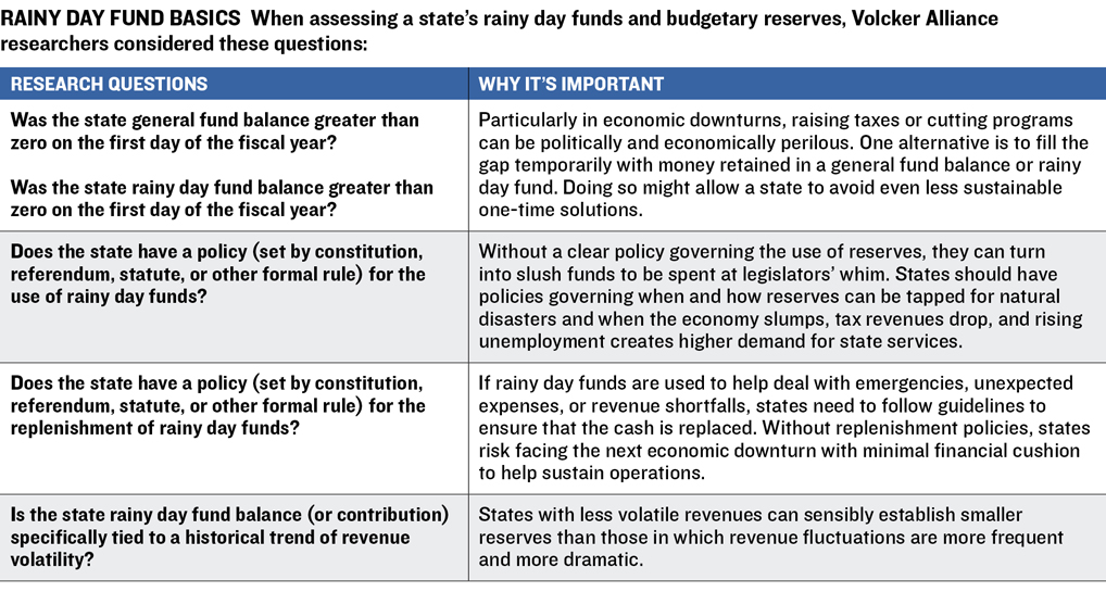
States should enact clear policies for deposits into and withdrawals from rainy day and other reserves. Without controls on withdrawals, spending decisions can be left to the whims of legislators or governors and result in increases in recurring costs rather than short-term infusions of cash for natural disasters or economic reversals. Without rules for replenishing rainy day funds, it can be too easy for legislatures to leave them empty or with minimal assets.
Montana is an example of a state that came up with answers to both challenges by creating a rules-based rainy day fund. The state depends heavily on volatile oil, natural gas, and coal production revenues; it also faces the constant risk of unexpected spending on wildfires and other natural emergencies. In 2017, it enacted legislation establishing a budget stabilization reserve fund to be used during a revenue shortfall. The first deposit of $45.7 million was planned for fiscal 2019. In the future, if general fund revenues exceed estimates by at least $15 million in a given fiscal year, half of the excess will be transferred into the rainy day fund on or before August 15 of the next fiscal period.
Prior to the new budget stabilization law, Montana had attempted to maintain a financial cushion with its year-end budgetary balances. But that did not provide the help the state needed in smoothing out volatile revenues. The creation of a rainy day fund, tying it to revenue volatility, and following best practices for its use and replenishment lifted Montana’s annual grade in this category to an A in 2018 from a D in fiscal 2016 and 2017. Its three-year average rose to a C.
TRANSPARENCY
States should provide the data that public officials, advocacy groups, and citizens need to thoroughly understand budgets. But while every state discloses budgetary information on websites, gaps remain, especially in the costs of deferred infrastructure maintenance and of tax expenditures. The latter, worth tens of billions of dollars or more every year, include the tax exemptions, abatements, and credits handed out for job creation, film production, research and development, and general subsidies such as eliminating levies on food and clothing sales. While GASB in 2015 began requiring all states and localities to show the cost of economic development incentives in their comprehensive annual financial reports, states should also report the value of these and all other tax breaks in budgets, as they are an expenditure of public resources. Yet the quality and quantity of disclosure varies from state to state.
Indiana is one of the states providing useful tax expenditure information that can aid in budget preparation and the evaluation of economic development programs. Under a law passed in 2015, the state’s Legislative Services Agency (LSA) is required to publish a detailed report on sales, income, and corporate tax expenditures in the fall of even-numbered years. The report published in late 2016 provided explanations of each tax expenditure, its history, and an estimate of its cost for each fiscal year of the upcoming budget.
A separate law passed in 2015 requires Indiana’s State Budget Agency to include a list of income and corporate tax expenditures in the report it submits to the legislative Budget Committee, also in the fall of even-numbered years, prior to debate over the upcoming biennial budget. That report, which uses data from both the LSA and the Department of Revenue, contains less explanatory detail but provides estimates for four years: the previous fiscal year, the current one, and both years of the upcoming biennium. The reports are intended to be complementary, with the much shorter budget agency publication geared for use in budget preparation and the legislative services report providing more detail on individual tax expenditures.
The addition of these reports raised Indiana’s 2018 transparency grade to B from a C in 2016 and 2017, though its three-year average remains a C.
When states adopt best practices such as these, we should not assume they will adhere to them indefinitely. In difficult fiscal times, legislators and governors can be tempted to forgo best practices and sacrifice fiscal stability for short-term fixes to maintain as many government services as possible. Yet states may find that long-term commitments to improved budget processes, especially in the areas highlighted in this study, will leave them better able to deal with the natural disasters and fiscal crises that inevitably occur.
Areas of Analysis
BUDGET FORECASTING
A state budget is as much a planning document as it is a financial one. The budget is intended to help a government remain fiscally sound and sustain its capacity to deliver services to the public. These goals may be unachievable if appropriate attention is not paid to estimating the possible future course of revenues and expenditures.
The use of a consensus method to estimate revenue is one of the best budget forecasting practices identified by the Volcker Alliance. The method attempts to avoid politically driven predictions by considering inputs from the executive and legislative branches and, sometimes, outside experts. Other best practices include providing a clear rationale to support forecasts and producing multiyear revenue and expenditure forecasts that can help policymakers spot and address long-term fiscal deficits. Yet only ten states received top average A grades in the budget forecasting category for fiscal 2016 through 2018, illustrating that most have considerable room to improve.
Among the findings:
- In 2018, nineteen states did not publish multiyear revenue forecasts in budget and planning documents covering at least three full fiscal years. That period is long enough to give policymakers a reasonable idea of potential fiscal trends.
- Twenty-seven states failed to present expenditure projections for the same period.
- Seventeen states had no multiyear forecasts for revenues or expenditures.
- Twenty-two states failed to use a consensus revenue estimate in the most recent year.
- Eight states did not provide a clear rationale to support their projections of revenue growth in the budget.
A few states are moving to improve their estimation processes, however. Utah, which received a three-year average of C in budget forecasting, passed legislation in 2018 requiring the Office of the Legislative Fiscal Analyst to prepare long-term budgets for programs appropriated from major funds and tax types. The law also requires regular stress tests showing how revenues and expenditures might be affected under different economic scenarios. Previously, the state produced no public long-term revenue or expenditure estimates. While the improvements were not enacted in time to raise the state’s 2018 grade, they point to an upward trend.
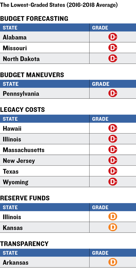
Meanwhile, Pennsylvania and New Jersey are considering adopting consensus revenue forecasts to replace the current ones, which are produced solely by the executive branch. But such reforms are not universal. In fact, twelve states scored D or lower, on average, over the three-year study period, with three—Alabama, Missouri, and North Dakota—receiving a D-minus, the lowest possible grade. North Dakota, for example, gives the governor exclusive authority for revenue forecasting. However, the legislature can change the number in the budget.
Some states use consensus forecasting yet fall short in other areas. For instance, Massachusetts relies by statute on consensus revenue estimates yet earned only an average C grade. On or before January 15, the state’s secretary of administration and finance must meet with the House and Senate Ways and Means committees to develop a consensus forecast of tax receipts for the next fiscal year’s budget. Massachusetts also provides a reasonable, detailed rationale to support revenue growth projections at the time of the initial budget. However, the state’s budgetary revenue and expenditure projections do not extend beyond the current fiscal year.
By contrast, Georgia, another C-graded state, produces both expenditure and revenue projections that extend three years past the current fiscal year, but it does not have a consensus estimating process. The governor’s office is responsible for producing the revenue estimate used in the proposed budget. The state does not disclose any rationale for the estimate, and any underlying assumptions for the estimate are not released publicly.
While most states need to improve aspects of their forecasting, some stand out for their exemplary procedures. One is Florida, the third-most-populous state and one of the ten with an average A grade. It has a consensus revenue estimating process that includes the Executive Office of the Governor, the Office of Economic and Demographic Research, and the Senate and House of Representatives. The estimation effort begins with a national economic forecast that is adjusted to a state outlook. Economists consider a variety of taxes, including the sales tax, which made up 63 percent of state tax collections in fiscal 2017, as well as other revenue sources, such as the corporate income levy, lottery and slot machine revenues, transportation revenues, and communications services taxes. Estimates are periodically revised with explanations of how and why revenues may be diverging from projections. Florida also holds estimating conferences that focus on demographic changes and spending categories, including criminal justice, education, social services, and the public employee retirement system. This level of transparency makes it difficult for the state to use one-time budgetary measures without, at a minimum, some form of public disclosure.
The consensus process for revenues and spending is intended to help the state meet its constitutional balanced budget requirement. Florida’s detailed, three-year consensus revenue forecast also comprises expenditure estimates that reflect budget baseline spending. In addition, a 2006 constitutional amendment requires the Legislative Budget Commission to produce a long-range financial outlook. In addition to providing projections, it considers critical needs, risks to forecast accuracy, and key budget drivers. The one released on September 14, 2018, covered fiscal 2019 through 2022.
Even states with severe fiscal challenges sometimes maintain forecasting practices that rank with the best. With the lowest general obligation bond rating of any state, Illinois has become synonymous with “broken budget process,” failing even to pass a budget in 2016 and 2017. Nonetheless, the state has statutory requirements for both the Governor’s Office of Management and Budget and the legislature’s Commission on Government Forecasting and Accountability to produce multiyear revenue and expenditure forecasts designed to help the legislature and governor know which future budget issues they may need to confront. The governor’s annual Economic and Fiscal Policy Report published in October 2017 includes national and state economic outlooks and provides projections of revenues, expenditures, deficits, surpluses, and liabilities through fiscal 2023.
Budgeting is not an exact science, and even states that score relatively well in the forecasting category can see forecasts miss the mark because of unanticipated events, errors, or changes in state law. Arizona, with a B average, publishes the rationale behind its revenue estimates, yet in 2017, the final year of a multiyear corporate tax reform plan, the state overestimated the amount of revenue the levy would produce. Starting in 2015, Arizona’s corporate tax rate was lowered in steps to 4.9 percent from 6.5 percent. But the 2017 receipts were about a third less than what had been estimated and budgeted.
Given the difficulty in making dramatic changes in budgetary practices, it is no surprise that most states retained similar annual grades from 2016 to 2018. But there were some exceptions. Texas saw its forecasting grade rise to B in 2018 from D in 2016 and 2017. This improvement followed a decision by the state legislature to experiment with long-term revenue and expenditure estimates. The General Appropriations Act for the 2018–19 biennial budget required the Legislative Budget Board to produce a report for the 2019 legislative session analyzing the impact of economic and demographic growth on state finances for ten fiscal years, starting in September 2019 and continuing through August 2029. The legislature will then evaluate the process.
While there are multiple best practices that contribute to a state’s quest for excellence in its budgeting, efforts to forecast future expenditures and revenues are particularly critical. If a state is far off on its expenditure or revenue projections, the very idea of a balanced budget becomes ever more elusive.
BUDGET FORECASTING
When States Make Midyear Budget Adjustments
States sometimes adjust their enacted budgets after the beginning of the fiscal year following an economic shock, such as a collapse in the housing market or drop in oil prices. Other times, however, midyear budgetary adjustments may be more a symptom of flaws in forecasting.
Though our 2017 report on state budgeting practices included the use of midyear budget adjustments in states’ annual forecasting grades, the 2018 report does not, as they usually show that policymakers are doing what is necessary to eliminate a shortfall. In fiscal 2017, sixteen states made such changes: California, Connecticut, Illinois, Iowa, Louisiana, Mississippi, Missouri, Nebraska, New Jersey, New Mexico, North Dakota, Oregon, South Dakota, Virginia, West Virginia, and Wyoming.
From July through October 2017 (the first four months of the fiscal year and the cutoff date for our 2018 report), only six states required midyear budget adjustments: Connecticut, Mississippi, Missouri, Montana, Nebraska, and Oklahoma. That number may not be a harbinger of the total number of states making adjustments in the fiscal year’s final eight months. Fiscal 2018 ended on June 30, 2018, for forty-six states. A final evaluation of budgetary processes covering the remainder of the fiscal year is scheduled to be published in 2019.
Mississippi, for example, with a three-year average of C in forecasting, made midyear budget adjustments in 2016, 2017, and 2018. In the first eight months of fiscal 2017, the state had a three-round series of cuts totaling $151 million. Part of this resulted from a $169 million overestimate of revenues and an accounting error made by legislators when writing the state spending plan. Among the agencies worst hit were the Mental Health and Health departments and the Mississippi Adequate Education Program.
California, meanwhile, did not require midyear budget adjustments in fiscal 2015 or 2016, or during the first four months of 2018. But a shortfall of $1.7 billion in general fund revenues in fiscal 2016 and 2017, stemming from overestimates of sales and corporation taxes, led to changes in the latter year. The shortfall was partly offset by upward revisions for personal income taxes.
Midyear budget adjustments may signal that projections were inaccurate, but they are not a bad practice in and of themselves. The frequent alternative is to resort to budget maneuvers, which have the effect of pushing shortfalls into future years, thus breaking a cardinal rule of good budgeting: matching a fiscal year’s revenues with expenditures in the same year.
It may be necessary to make midyear adjustments to avoid deficits and preserve bond ratings. But states should make them with care to avoid damaging effective programs.
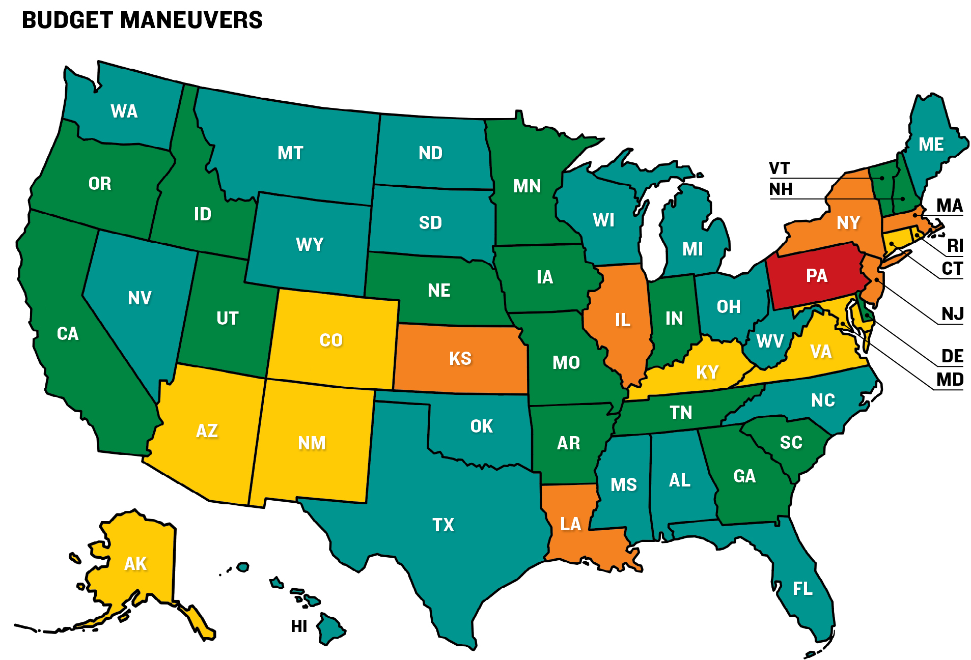
Budget Maneuvers
Fiscal sustainability is key to successful budgeting. Using one-time actions to balance a budget will produce shortfalls in future years unless recurring revenues are increased or expenditures reduced. Similarly, deferring payment of planned expenditures to a future fiscal year can prompt a state to use maneuvers to pay for past-due bills.
In the 2018 evaluation, about the same number of states have had improvement in the budget maneuvers category as have had their grades decline.
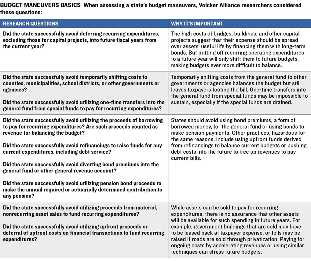
We asked nine questions to determine how states should be graded in their use of budget maneuvers, or one-time actions, to offset continuing expenditures. They fall into four groups of activities: deferring recurring expenditures; moving costs from the general fund to other public entities or raiding special funds to prop up the general fund; funding recurring expenses with debt; and shifting revenues to the current year from the future or selling long-lasting assets to pay the current year’s bills. Three-year average state grades were widely spread. Sixteen scored an A; eighteen got a B; nine were given C; six received a D; and only one, Pennsylvania, got the lowest grade possible, a D-minus.
One budget maneuver that contributed to Pennsylvania’s low grade was a decision to use $1.5 billion in proceeds from the issuance of bonds secured by the 1998 Tobacco Master Settlement Agreement—a legal settlement between cigarette producers and forty-six states, the District of Columbia, and several territories—to help offset a negative general fund balance at the end of 2017. Massachusetts earned an average grade of D, the second-lowest mark. It has relied heavily on maneuvers to offset a long-term disconnect between revenues and expenditures: It passed tax cuts in 2000 without sufficiently reducing spending or sufficiently growing its economy to close the resulting gap. When revenue forecasts are higher than actual receipts or expenditures are higher than original estimates, states may turn to one-time actions to address budgetary shortfalls.
The use of budget maneuvers accelerates in times of economic stress and tends to decrease when the economy is improving. Although it finished fiscal 2017 with a budget surplus, Louisiana dealt with a revenue shortfall during the year by moving money from its rainy day fund and other special funds to the general fund to pay for ongoing expenditures. The state also used cash generated from a bond refinancing to cover operating costs in fiscal 2017, although less than it did in 2016. Further, $61 million in planned Medicaid spending deferred in 2016 was deferred again to fiscal 2019. Nonetheless, the state’s grade in the category rose to C in 2018 from D in 2016 and 2017, though its average is still D.
Other budget maneuver findings for fiscal 2016 through 2018 include:
- Forty-five states avoided funding recurring expenses with debt in 2018. The five states that used the technique were Alabama, Connecticut, Illinois, New Mexico, and Pennsylvania. Each of those states also used debt for recurring expenses in 2017, as did Louisiana and Rhode Island.
- No state issued bonds to make actuarially determined contributions to public employee pensions.
- Only two states—New Jersey and Illinois—projected asset sales to support recurring expenditures and help keep their budgets in balance in 2018. Illinois added $300 million to its budget from the proposed sale of the Thompson Center, a Chicago complex that houses state offices, stores, and restaurants, although the sale plan was later shelved. The New Jersey budget relied on $325 million in asset sales, including $321 million from the sale of excess broadband capacity.
Five states that achieved a three-year A average did so with improvements from 2017 to 2018: Arkansas, Indiana, Iowa, Oregon, and Vermont. Revenue shortfalls led Iowa to use $25.1 million in interfund transfers to shore up the general fund in fiscal 2017—an action not needed in 2018. Vermont deferred spending by delaying until fiscal 2018 the outlay of $16.3 million of corporate refunds expected to be paid in fiscal 2017. This technique brought its overall grade in budget maneuvers to a B in 2017. The state didn’t use similar shifts in fiscal 2018, however, which elevated its grade to an A.
Still, twenty-nine states transferred cash to their general fund from special funds in 2018, including Illinois, New York, Ohio, Pennsylvania, and Texas.
Among states deferring recurring expenditures into future fiscal years from the current one was New York, which borrowed $215 million from the New York Power Authority in March 2009 and was supposed to repay the loan by September 30, 2017. But in fiscal 2017, an amendment to the memorandum of understanding extended the payment plan until fiscal 2023. In fiscal 2018 it paid back $22 million, leaving $193 million deferred to the following five years. The state also borrowed $103 million from the authority in September 2009, which was to be repaid by September 30, 2014. But that payment had been similarly extended to a series of installments between fiscal 2015 and 2019.
Maneuvers often receive little attention in budget discussions. Governors and legislators frequently talk about streamlining and efficiency as the cure for expenditures that outstrip revenues. But while the latest plan to restructure government is debated, states often turn to one-time actions for short-term fixes that actually may need to be repeated again and again.
BUDGET MANEUVERS
The Fund Transfer Trap
When Volcker Alliance researchers scrutinized states’ use of maneuvers to balance their budgets, the most widely used technique was making one-time transfers to the general fund from special funds to pay for recurring expenditures. Twenty-nine states engaged in this practice in fiscal 2018. While this indicates that these states are most likely caching spare cash in numerous places other than their official rainy day fund reserves, it poses a threat to the use of funds earmarked for specific purposes—say, clean energy retrofits or transportation. Additionally, reliance on fund transfers to balance budgets may not be repeatable indefinitely if the special funds are drained until they run dry.
Of the ten largest states by population, only California, Georgia, and Michigan eschewed such transfers in fiscal 2018. And while California and Georgia also avoided transfers in 2016 and 2017, Michigan broke ranks after the state Senate passed a bill permitting a one-time transfer to the general fund from the unemployment contingency fund, which is made up primarily of penalties and interest paid to the state because of fraud.
California has not always had such a clean record; it still carries liabilities from engaging in maneuvers in previous years. The state Department of Finance estimated that the balance of general fund liabilities to special funds was about $1.4 billion as of June 30, 2017.
Transfers involve significant sums in some states. New Jersey’s D average in budget maneuvers is largely due to its consistent use of this technique for all three years studied. In its fiscal 2018 budget, the state continued its longtime use of clean energy funds for general fund purposes, with the transfer of $161 million. There was a similar transfer of funds—totaling $204 million in the year—from the New Jersey Turnpike Authority to the general fund to help cover the operating expenses of New Jersey Transit, the state-owned commuter rail and bus system.
Similarly, Kansas shifted $198.4 million and $118.8 million in fiscal 2017 and 2018, respectively, to the general fund from the Pooled Money Investment Portfolio, which is made up of money from state agencies, local governments, and school districts and is invested by a state board. The funds are scheduled to be repaid over six years. With a three-year average of D in the category, Kansas has also made regular transfers of highway funds to the general fund, ranging from $173.5 million in 2015 to $288.3 million in fiscal 2018. The state may be able to lessen dependence on transfers and other budget maneuvers following a 2017 restoration of tax rates to the pre-2013 level.
In fiscal 2018, the New Mexico Senate raised recurring general fund expenditures by $90.1 million, using $81.4 million in transfers to cover most of that increase. Among the transfers, $71 million came from money that would have gone to the Severance Tax Permanent Fund, and $10.4 million came from the suspension of a severance tax bond distribution to the state water project fund.
Transfers from special funds are a particularly seductive approach to balancing a budget. They are nearly invisible without an exacting analysis of the budget and do not frequently show up in headlines. Still, they cannot go on indefinitely and may ultimately leave a state confronting a shortfall that can’t be fixed so quietly.
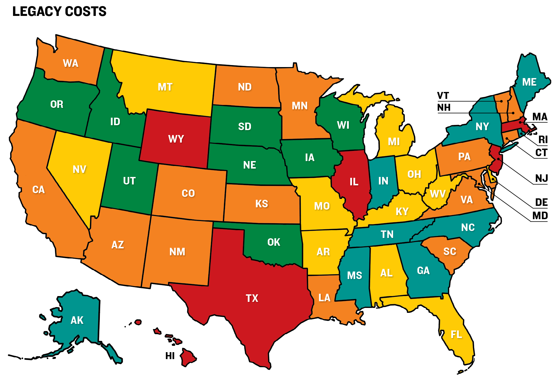
Legacy Costs
Trillions of dollars in unfunded liabilities for state public worker pensions and other postemployment benefits (OPEB), largely retiree health care, represent unpaid costs for services that governments delivered in the past. Efforts to cover these legacy costs present many states with challenges that often elude easy solutions, and the costs increasingly threaten to crowd out spending on education, infrastructure, and other critical needs.
While a 19 percent gain for the Standard & Poor’s 500 Index in 2017 helped state pension funds reduce their deficit by a small amount from the previous year, they still had a $1.35 trillion gap, according to data compiled by Bloomberg. This deficit was 6.5 percent larger than it was in 2015. Put another way, states in 2017 had set aside only $2.95 trillion to cover pension obligations totaling $4.23 trillion. On top of their pension obligations, states posted OPEB liabilities of $692 billion in 2016, the most recent year for which data are available, while amassing just $46 billion in assets. Perhaps it is not unexpected that in the legacy costs category, only eight states received average A grades for 2016 through 2018, while twenty-two were graded D or worse.
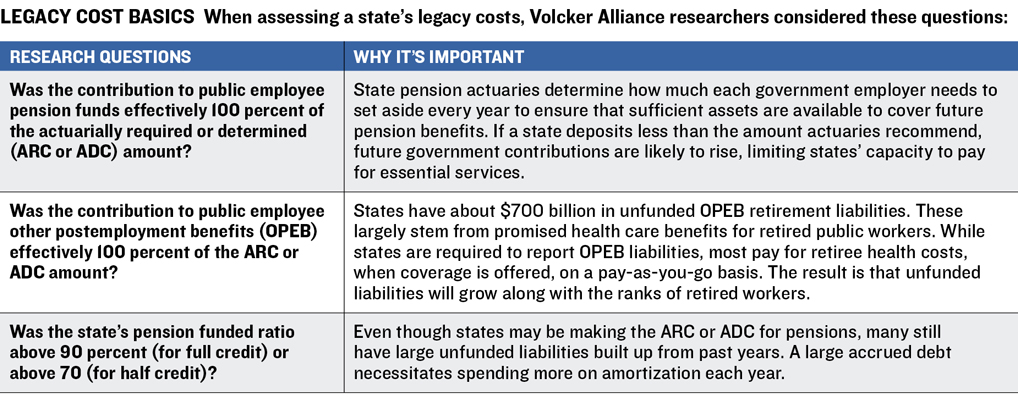
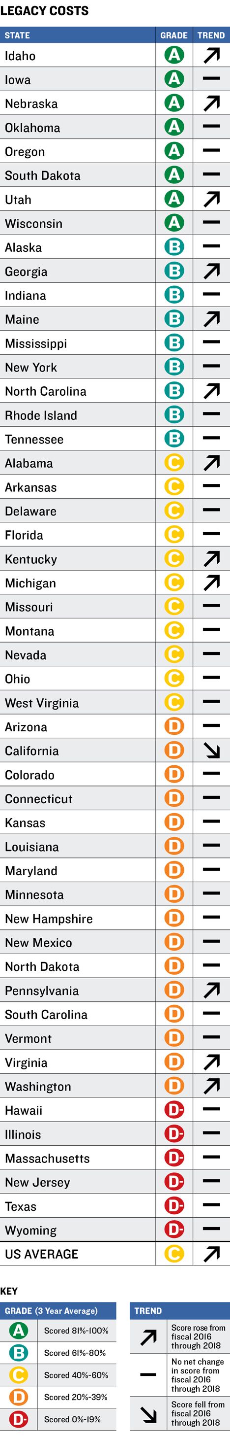
When calculating annual grades for legacy costs, we considered a state’s demonstrated willingness to meet pension obligations and OPEB. Thirty percent of the overall category grade was determined by a state’s making its actuarially required or determined contribution (ARC or ADC) for OPEB. Seventy percent of the grade was based on whether the state had made its public employee pension ARC or ADC and on its pension funding ratio—the amount of assets available to cover promised benefits—as of 2017.
The eight states receiving an average of A in legacy costs were Idaho, Iowa, Nebraska, Oklahoma, Oregon, South Dakota, Utah, and Wisconsin. Six states received the lowest possible grade of D-minus: Hawaii, Illinois, Massachusetts, New Jersey, Texas, and Wyoming. Each of these states failed to make their full ARC or ADC for both pension and OPEB in either 2017 or 2018.
With the US economy in its tenth year of recovery from the Great Recession, states generally did better on making their full annual pension contribution in 2017 and 2018 than in previous years. In 2015, sixteen states failed to make the full contribution, versus fifteen in 2016 and twelve each in 2017 and 2018. Pennsylvania’s D-minus grade in 2015 and 2016 rose to a D in 2017 and 2018. In those two years, the state made its full annual contribution to its two major pension systems. Still, the many years that Pennsylvania skimped on its contributions left it with a funding level of 55.3 percent in its most recent actuarial valuation, down from 127 percent in 2000.
Kentucky, the state with the lowest pension funding ratio in 2017 (33.9 percent), also saw its grade improve from a three-year D average in last year’s report to a C average, largely because it fully funded its annual employer pension contribution in fiscal 2017 and 2018. This was not the case in 2015 or 2016 because of state underfunding of the annual contribution for the teacher pension.
Several other states that are now making 100 percent of their actuarially determined annual pension payments are still less than 70 percent funded because of past contribution shortfalls, market losses, or both. Connecticut is an example. On an annual basis, its pension fund contributions were 98.3 percent of the ADC in 2017, but its pension funding level was only 43.8 percent. Coupled with its neglect of actuarially required annual funding for OPEB, this resulted in a D for the state in legacy costs. The same was true for New Hampshire, which made its full annual pension contribution each year of the evaluation but did not provide full annual funding for OPEB and had a pension system that was only 62.6 percent funded.
Thirty-eight states got credit for making their full annual pension contribution, while only twenty did similarly for OPEB. This number included some states, including Indiana, Nebraska, Iowa, and Oklahoma, with minimal OPEB benefits. As a result, they do not face fiscally draining long-term costs in this area. (Some states received credit for pension or OPEB funding if the unfunded portion of the ARC or ADC was under $50 million and less than 0.5 percent of the budget.)
The long-term liability is significant for states providing substantial direct subsidies for retiree health care. New York, for example, had a $72.8 billion unfunded actuarial accrued OPEB liability in 2016. To fully fund that obligation over time, including the amount necessary to cover the cost of benefits earned in the current year and to amortize the unfunded liability, the state would have needed to pay $3.2 billion in fiscal 2017. It contributed only 44 percent of that amount, $1.4 billion, which covered the current-year costs for retirees. By failing to fund OPEB as actuaries recommended in 2017, New York added $1.8 billion to its long-term liability.
One state that improved its OPEB funding practices in this year’s evaluation was Georgia, which received an annual grade of C in 2015 and 2016 and A in 2017 and 2018. Georgia’s 2015 evaluation showed minimal assets for the state or school OPEB funds, leaving it with an unfunded liability of nearly $14 billion. The state began to prefund OPEB in fiscal 2016, and the following year it made sufficient contributions to its state and school plans to match actuarially determined amounts. While this indicates progress, the state has not instituted statutory policies committing it to continue contributing at levels that will lead in the long term to a fully funded OPEB trust.
Courts, interpreting state constitutions or statutes, have typically made it easier to alter OPEB benefits than pensions. For instance, in 2018 an appellate court permitted New York to increase the contributions that New York State Thruway Authority retirees contribute for health care.
Pensions are more generally regarded as binding contractual or even constitutional obligations and have been far more difficult to alter for current employees. And while pension obligation bonds, such as those previously used by Kansas, Illinois, and New Jersey, can raise money to lower unfunded liabilities, they merely shift debt from one arm of government to another. For states such as these, devising a durable strategy to cover retirement promises made to public workers while continuing to provide essential services is a truly arduous task.
LEGACY COSTS
How States Created Today’s Pension Funding Gaps
State pension system shortfalls are often the result of decisions made years or decades ago.
In 2017, twenty-one states had pensions that were less than 70 percent funded. That stands in contrast to 2000, when half of state plans were at least 100 percent funded. Many states’ pension plans saw funding levels drop when technology stocks declined dramatically in 2000. The Great Recession had an even larger impact. Many states increased retirement benefits in the 1990s and early 2000s in lieu of salary increases, but not all of those raised government or worker contributions sufficiently to finance the additional largesse.
From 1997 to 2006, thirty-two states failed to make their full or nearly full actuarially determined or recommended annual pension contribution in at least one year. The shortfall left the underpayment to be addressed subsequently and the unpaid sums to compound at the funds’ assumed rate of return—currently about 7.5 percent. From 2016 to 2018, the years covered by this study, sixteen states missed making the full contribution in at least one year.
Kentucky and New Jersey are extreme examples of a precipitous drop in pension funding ratios. Both were at least 100 percent funded at the end of the twentieth century, but as of June 30, 2017, the unfunded liability for Kentucky’s pension systems was $42.9 billion, while New Jersey’s was $142.3 billion. That translates into a funding ratio of 33.9 percent and 35.8 percent, respectively.
New Jersey began steadily losing ground in its Public Employees’ Retirement System and Teachers’ Pension and Annuity Fund at the start of this century. But the state’s problems began even before that, when Governor Christine Todd Whitman signed into law the final part of a 30 percent income tax cut in 1995.
To make up for the revenue decline, the governor reduced the amount of money contributed to the pension funds and in 1997 sold $2.8 billion in pension obligation bonds at just under 8 percent interest. A plunge in stock prices between 2000 and 2002 consumed part of the funds raised through the debt sale, and New Jersey will continue to pay about $500 million annually in debt service costs for those bonds through 2029.
Despite the market losses, the state boosted pension benefits by 9 percent in 2001—without any plans for covering the additional cost. In fiscal 2018, New Jersey temporarily shifted ownership of the state lottery and its proceeds to the retirement funds for teachers, public employees, and police officers and firefighters. The move made the pension system appear better funded, but the net amount being injected by the state is not scheduled to reach the ARC level until fiscal 2023. The shortfall continues to deprive the pension system of any possible earnings on the sums that actuaries say should be contributed.
Kentucky has a similar story. In 2002, the Kentucky Retirement Systems, comprising five separate pension plans, was 100 percent funded. But starting in 2004 annual contributions ran consistently short of actuarial recommendations. The biggest problem was the state employee plan for those in nonhazardous jobs. At the height of the ARC underfunding, in fiscal 2012, the employer annual contribution for that plan fell short by $226.3 million—half of the actuarial recommendation. The legislature passed a bill in 2013 mandating full annual contributions for the Kentucky Retirement Systems. In the biennial budget that began July 1, 2016, and ended June 30, 2018, the state exceeded the ARC.
The state is still grappling with underfunding that stems from past actions. These actions include using an accounting process that allowed the state to backload its ADC so that costs would grow over time, using assumptions that turned out to be overly optimistic, and providing annual cost-of-living increases to retirees for decades without adequate plans for funding them. This occurred most recently in 2011. Two years later, legislators eliminated cost-of-living adjustments (COLAs) except in years when the assets of the system are greater than its liabilities. Still, just between 2008 and 2011, unfunded COLAs added $1.45 billion to the unfunded liability of the Kentucky Retirement Systems.
Reserve Funds
Recessions, commodity price swings, and natural disasters can wreak havoc on state budgets. Because states lack the federal government’s ability to print money, they try to maintain reserves, usually known as rainy day funds, as their bulwark against crisis-driven budget shortfalls.
Although a few states lack rainy day funds or have ones that are practically empty, the economic recovery that began in 2009 has helped most states restock their vaults with cash. At the end of fiscal 2018, the median state had reserves of 5.8 percent of general fund expenditures, the largest cash trove since rainy day funds hit a recent low of 1.9 percent in 2011, according to the National Association of State Budget Officers.
Destruction caused by Hurricane Florence in September 2018 demonstrates how critical rainy day funds can be for fiscal management. After the storm struck North Carolina, legislators authorized the drawdown of $756.5 million from the state’s $2 billion savings reserve—as its rainy day fund is known—to help finance recovery. The total cleanup bill was estimated at $850 million, or 3.6 percent of the fiscal 2019 general fund budget, according to Moody’s Investors Service.
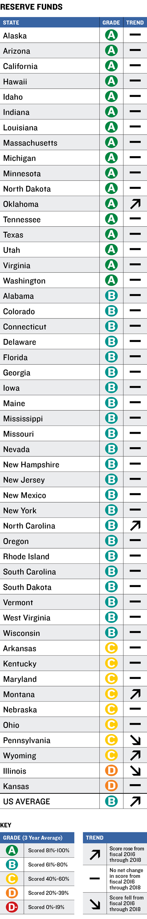
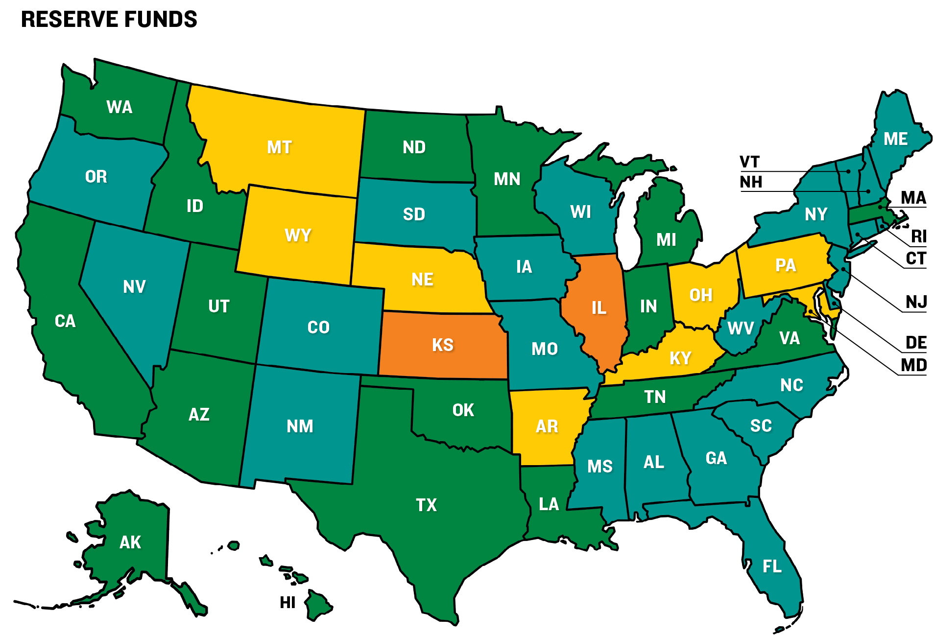
North Carolina, which received an A in the reserve category in 2018 and a three-year average of B, has reserves that have grown tenfold since the Great Recession. In fact, with economies and revenues gaining, most states earned favorable grades in the broad category of reserves. Seventeen states had A grades for their three-year average; twenty-three received a B; eight were given a C; and two, Illinois and Kansas, trailed their peers, each with a D.
Forty-five states reported a positive balance in reserve funds in fiscal 2018. The five others, which have no or minimal reserves, were Illinois, Kansas, Montana, New Jersey, and Pennsylvania.
General fund reserves, which may be easier to tap than rainy day funds, also play a role in fiscal stability. Forty-one states had positive general fund balances on the first day of fiscal 2018. The only states without money in a rainy day fund and with a minimal or negative general fund balance at the beginning of fiscal 2018 were Illinois and Pennsylvania. Illinois got a D in the reserve fund category and Pennsylvania received a C.
Our assessments of state reserves include more than maintaining a rainy day fund or an equivalent. States need to have clear policies governing fund withdrawals. And while a drawdown of rainy day funds is a one-time revenue action, the impact of the maneuver can be mitigated if a state maintains a clear policy for fund replenishment. States should also establish a formal connection between reserve fund levels and historical revenue volatility.
Pennsylvania’s grade was lifted by its guidelines for the disbursement and replenishment of money from its reserve fund, even though the state had virtually no money in the kitty in fiscal 2017 and 2018. Illinois would have received a D-minus instead of a D save for the fact that it has policies for replenishing its rainy day fund. In years when revenues grow 4 percent or more, the state’s Budget Stabilization Act limits the annual appropriation and requires a deposit to the reserve. But in fiscal 2017 Illinois’s rainy day fund would have covered the state’s needs for only two hours, according to Comptroller Susana Mendoza.
Forty-three states got credit for maintaining disbursement policies for their rainy day funds, and all but two—Arkansas and Kansas—had replenishment policies in 2018.
New York, which got a three-year average of B in the reserves category, is among the states with specific guidelines for the appropriate use of reserve funds. That money can be used during an economic downturn, which is defined as five consecutive months of decline in a composite index the state calculates. The fund can also be used in the case of a catastrophic event, such as a hurricane.
Ohio has been building its rainy day fund even though revenues have been below expectations. General fund tax revenues were 3.7 percent lower than anticipated, or $849 million, for 2017. The Ohio budget stabilization fund was 5.8 percent of general fund spending at the end of 2017, down slightly from the 2016 level but otherwise at its peak since 2010. At the beginning of the current fiscal year, the fund had reached 8.5 percent of spending. Still, Ohio, with a three-year average grade of C, lacks reserve policies that consider revenue volatility. The state also only loosely specifies conditions for use of the rainy day fund.
Nineteen states maintain a formal tie between revenue volatility and reserves. They recognize that their tax structures and economies influence the amount of money they need to save; the more that revenues vary from year to year, the greater the reserve should be.
California, with a three-year average grade of A, exemplifies a state with volatile revenue, in large part because of the extreme progressivity of its income tax system, a concentration of high-income taxpayers, and strict educational spending mandates that limit overall spending flexibility. The state has attempted to cope with revenue volatility through a 2014 ballot measure requiring that a portion of capital gains tax revenue be deposited in the rainy day fund when income from the levy exceeds 8 percent of general revenue. This helps the state build up its reserve when financial markets are strong and prevents it from spending large influxes of capital gains dollars that won’t be available when the economy weakens.
One of the most difficult challenges presented to state policymakers is to ensure that they are structuring finances to be countercyclical. Flush times should not provoke overspending, and hard times should not lead to reliance on gimmickry to avoid severe spending cuts. Rainy day funds and year-end general fund balances are two of the tools that help states keep their finances in order through the downward portion of economic cycles.
RESERVE FUNDS
Building Revenue Volatility into Rainy Day Fund Rules
For at least three decades, many states have followed a general rule that rainy day fund reserves should equal about 5 percent of the general fund balance. While the origins of this rule remain uncertain, it has become clear that it makes little sense to hold all fifty states to the same reserve standard without considering their individual revenue structures.
Largely due to advocacy efforts by the Pew Charitable Trusts, a growing number of states have acknowledged this issue and are tying their rainy day fund goals to the volatility of their revenue streams. Nineteen states follow this practice, thanks in part to recent legislative momentum. In 2017, Hawaii, Maryland, Montana, New Mexico, North Carolina, and North Dakota changed rainy day fund policies to increase their consideration of revenue volatility.
States with more or greater swings in revenue are more likely to need larger reserves. The Great Recession clearly showed states that they were unprepared for the extreme drops in revenue that were in part attributable to a highly volatile revenue stream.
For example, in November 2016, Maryland’s comptroller, and departments of Budget and Management and Legislative Services released a joint study looking at the state’s volatile revenue structure and recommending changes to its reserve fund policies. A bill passed in the 2017 legislative session that takes effect in 2020 will direct a portion of capital gains and other non-withholding income tax revenue to Maryland’s rainy day fund and, when reserve fund caps are reached, to a newly created Fiscal Responsibility Fund. The latter can be used for pay-as-you-go capital projects or allocated to state trust funds with unfunded liabilities.
One group of states with particularly fragile revenue streams are western ones, including Alaska, Montana, North Dakota, and Wyoming, that rely on severance fees and taxes on the production of oil, gas, coal, or other natural resources to help pay for services. Understandably, all four states connect funding of reserves to revenue volatility. The North Dakota legislature changes the rate of contribution to its fund based on annual revenue collection, which is closely connected to oil prices.
Some states that tie their rainy day fund policies to revenue volatility also cap the amount they are allowed to contribute, a practice that may partially negate the purpose of the volatility link. Virginia, for one, uses historic revenue growth in its major tax categories as an important factor in making decisions about its rainy day fund. This was a successful formula in the mid-2000s, driving large deposits during a time of economic expansion. But the state had a 10 percent cap on total deposits, a point it reached in fiscal 2006 and 2007. The reserve enabled the state to cover just 15 percent of the shortfalls that occurred between 2008 and 2010. Virginia voters in 2010 approved a measure raising the cap to 15 percent, which would have given it an additional $594 million to face revenue losses and spending demands during and shortly after the Great Recession.
There is a good reason a growing number of states are tying the amounts held in rainy day funds to volatility rather than keeping a set percentage of general fund revenues on hand. The practice helps avoid salting away too much cash in states that have a less volatile tax structure or skimping on reserves in states likely to experience more revenue swings.
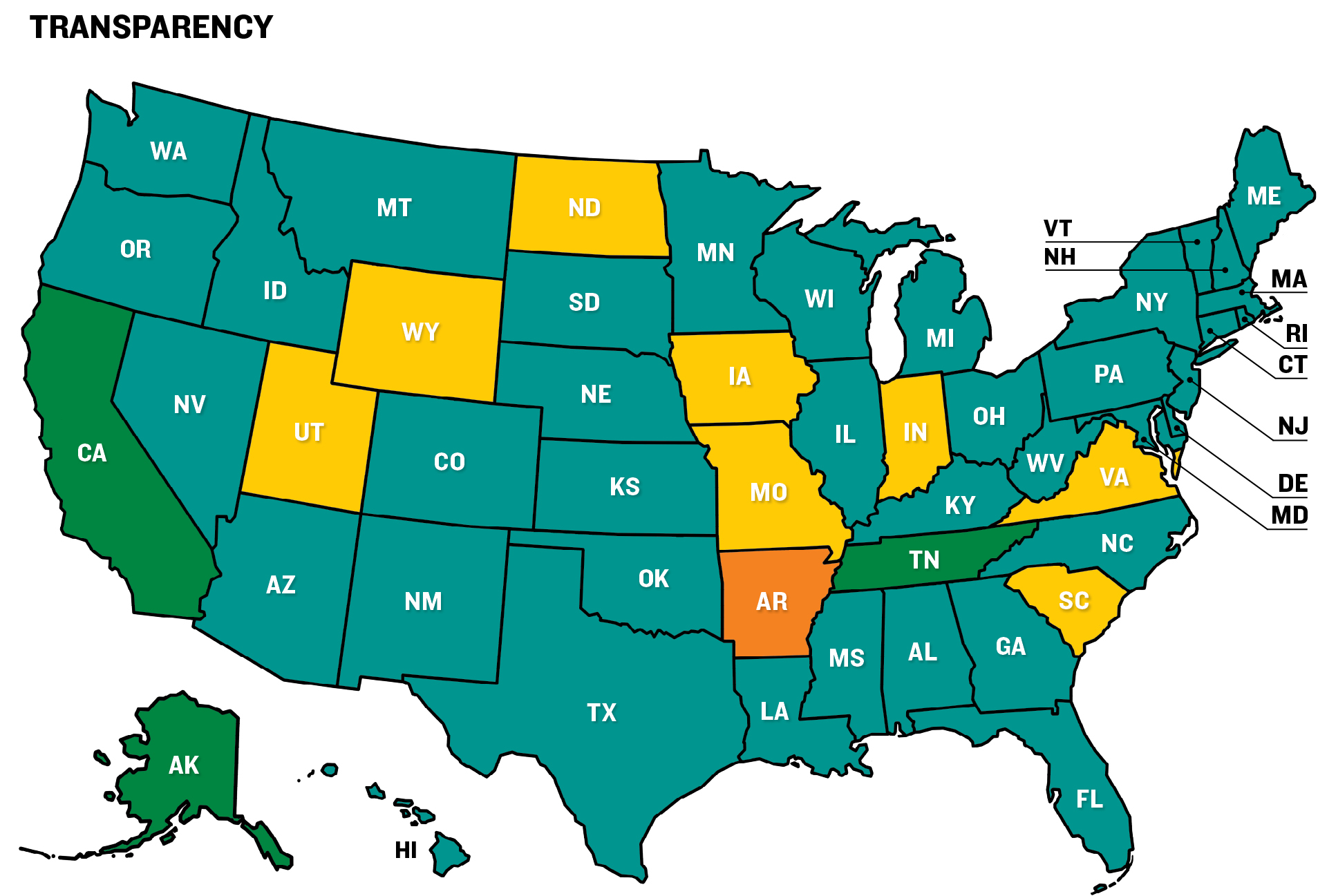
Transparency
Budget information is worth little to elected officials, policy advocates, and the public if they can’t find it. Yet only three states won top average A grades for fiscal 2016 through 2018 for budget transparency. The lack of comprehensive budgetary information on the cost of deferred infrastructure maintenance in forty-six states explains part of the result, but many states also trail in other critical areas.
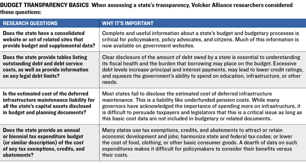
In addition to the infrastructure disclosure, a state budget transparency strategy should include a consolidated website that provides easy access to budget procedures and timing. It is also important to post links to information needed to form spending plans, such as reports on unfunded liabilities for long-term pension or retiree health care, capital budgeting, economic forecasts, or reserves. To follow best practices, states should also produce clear, accessible, and detailed tables of outstanding debt and debt service costs, and an annual or biennial accounting of the cost of tax exemptions, credits, and abatements. The good news is that thirty-eight states received a B average for the three-year period, showing reasonable efforts at disclosure in these areas.
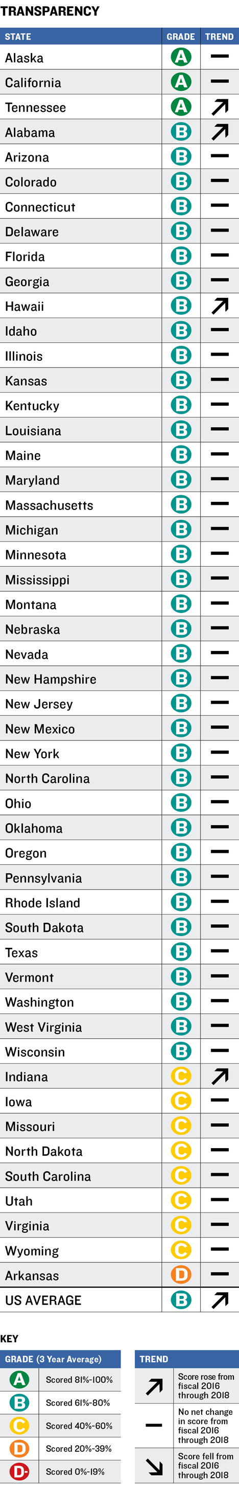
None earned the lowest mark of D-minus, and only Arkansas received a D. The state lacks a consolidated website that provides budget and other financial information essential in developing and analyzing its biennial spending plan. Like most other states, Arkansas does not disseminate any information about deferred infrastructure maintenance liabilities. It also does not publish a capital budget, although some information about capital expenditures can be obtained from individual appropriations bills or the state’s transparency website.
While federal standards for reporting highway and bridge deferred maintenance costs are being upgraded, Hawaii, which received a grade of B, and the three states receiving top average scores of A—Alaska, California, and Tennessee—are the only ones making a clear effort to disclose these costs in budgetary or related documents.
Alaska’s Legislative Finance Division reports the cost estimates by department and agency, estimating a $1.9 billion deferred maintenance backlog for its 2,200 facilities as of January 2018. California, meanwhile, produces the data in an annual five-year infrastructure plan as part of its budget documents. The state estimated $78.1 billion in deferred maintenance costs in 2017. The Tennessee Advisory Commission on Intergovernmental Relations, created by statute in 1978, handles that state’s deferred maintenance cost disclosures. We gave Tennessee a three-year average of B in transparency in our 2017 report because of a lack of deferred infrastructure maintenance disclosure in budget documents. However, we have found that the commission’s reports are equivalent to budgetary disclosures.
The absence of deferred maintenance cost information in most states is a critical shortcoming in a nation in which the word “infrastructure” is frequently preceded by “crumbling.” Unfunded infrastructure maintenance is akin to underfunded pensions; the total liability for each may grow every year that spending is short of what is required. A road needing only partial resurfacing in a given year may be costlier to repair—and result in congestion and higher car and truck maintenance expenses—if work is repeatedly put off. Similarly, the usefulness of buildings and other public assets declines, and long-term costs rise, if the state does not provide necessary upkeep.
Other transparency findings for fiscal 2016 through 2018 include:
- Eight states failed to provide an annual or biennial tax expenditure budget or equivalent report showing the cost of state-provided exemptions, credits, and abatements. But Indiana raised its 2018 transparency grade to B from C by requiring the Legislative Services and the State Budget agencies to produce complementary tax expenditure reports, with the shorter budget version to assist in biennial budget formation and the legislative report to delve into greater detail on each tax expenditure. The first reports were produced at the end of 2016. (Since the reports were released following adoption of the 2016–17 biennial budget, the state received no credit for the document in 2016 or 2017, leaving its three-year average unchanged at C.)
- All states provided tables listing outstanding debt and debt service costs, as well as information on any legal debt limits.
While most states have consolidated budget websites and were given credit for them in their evaluations, their content and usefulness vary.
On the Arizona Governor’s Office of Strategic Planning and Budgeting website—the state received a B average in transparency—it was a simple matter to find past budgets and supplemental information. It was also easy to locate budget briefs, which present summarized revenue and expenditure information with straightforward charts and explanations of how spending plans link to the governor’s priorities. The consolidated website helps users track monthly spending, provides links to five-year strategic plans, chronicles the impact of court cases on the state budget, and posts updates to revenue projections, such as a budget director memo from April 2018 noting that fiscal 2018 revenues were $262 million over projections.
In Ohio, which also scored a B average in the category, the Office of Management and Budget provides a web page with links to many standard features, including the operating and capital budgets, detail on the budget stabilization fund, and monthly financial reports. One feature, Ohio’s Interactive Budget, lets users click through a series of charts for more information derived from the state’s accounting system. Users can get levels of detail on such questions as the breakdown of nontax and tax revenues and the portion of the budget spent on various items, including debt service, personnel, and equipment.
Other states that received credit for having a consolidated budget website may still scatter other information over different sites. Take Nevada, which earned a three-year average of B in transparency. The governor’s Finance Office website presents elements such as the executive budget, agency budget requests, information on performance-based budgeting, and an explanation of the Economic Forum, which produces the state’s consensus revenue estimate. Information on debt, however, appears in the annual report of the separately elected state treasurer, which includes a summary of the activities of the Debt Management division. A key debt capacity and debt service report for 2017 to 2019 is even more difficult to find and appears to be available only on the state Senate Finance Committee website, embedded in meeting notes.
Similarly, the quality of tax expenditure reports varies among the forty-two states that received credit for following this best practice. Some states that did not receive credit for producing such reports provided partial information but failed to include comprehensive reports on a consistent basis. From 2007 to 2011, the Virginia legislature required the Department of Taxation to report the fiscal, economic, and policy impact of sales and use tax exemptions. The requirement was repealed in 2012. Though the legislature’s Joint Subcommittee to Evaluate Tax Preferences currently publishes updates on the topic on its website, disclosures are neither consistent nor complete—one of the reasons Virginia received only a C average for transparency.
Despite not capturing credit in this study for producing an annual or biennial tax expenditure document, Iowa has instituted processes that result in the regular production of reports designed to provide state officials with insight into forgone revenues. While the state passed legislation in 2012 to increase the frequency of formal tax expenditure reports to annually from every five years, it has not produced the document in recent years. However, it has provided information on the top twenty sales and use tax expenditures for fiscal 2017.
State and local governments are likely to continue to improve their tax expenditure disclosure to comply with GASB Statement No. 77, which became effective for financial reports covering periods that started after December 15, 2015. The state requires governments to disclose in their CAFRs any tax abatements granted to individuals or companies, generally for economic or real estate development. The disclosures include the amounts involved and any commitments made by companies receiving exemptions.
Because of timing issues, there are limits to the new rule’s usefulness in budgeting. In most states with annual budgets, fiscal 2018 budget preparation began in fall 2016, while the most recent CAFR covered fiscal 2015. In addition, GASB 77 covers only certain kinds of abatements—those that occur in exchange for agreeing to a specific action, such as creating a set number of jobs. Tax exemptions or credits that are more generally available, such as sales tax exclusions for groceries or property tax abatements for nonprofits, are not included.
States can underestimate the importance of transparency. It can be a costly exercise, requiring frequent updates of websites and compilation of data. But making important fiscal decisions without easily available data contributes to weaknesses throughout the fiscal system.
TRANSPARENCY
The Ins and Outs of Tax Expenditures
Federal, state, and local governments devote billions of dollars in public resources to tax expenditures. These include exemptions, deductions, credits, and other exclusions from levies that would otherwise be paid by individuals or businesses.
While many such expenditures by states are focused on economic development and jobs, they also may be aimed at reducing the cost of basic consumer necessities such as food and clothing, subsidizing low-income senior citizens or veterans, or bringing deductions in line with those in the federal tax code. While forty-two states provide at least some regularly updated information on tax expenditures, their reports vary in scope.
Tax expenditure reports should be used to measure the costs of the abatements against their benefits, thus helping government officials and policy advocates evaluate which programs should be curtailed, maintained, or expanded. They should be produced annually or biennially and be publicly available on budget websites, or on easily accessible transparency or revenue department sites.
A useful state report includes comprehensive data pertaining to all major streams of tax revenue, including personal and corporate income taxes, sale and use taxes, real and personal property taxes, and excise and gross receipts taxes.
Georgia, which has a three-year B average for transparency, has one of the more complete reports. Published annually, it is available on the website of the Governor’s Office of Planning and Budget. It does not provide the total value of tax expenditures but does show estimates for three fiscal years for hundreds of credits, exemptions, and deductions for individuals and companies. The comparative fiscal year data enable readers to see how the amounts involved change from year to year. For instance, the fiscal 2018 report shows that the film tax credit cost the state $414 million, up 22 percent from 2016.
Ohio is another state winning a B. Its comprehensive tax expenditure report is published as Book Two of the biennial budget and can be found on the Office of Budget and Management website under Operating Budget. The report for the 2018–19 biennium, released in November 2016, includes estimates for fiscal 2016 through fiscal 2019. It lists $9.1 billion of tax expenditures in fiscal 2018, about 28 percent of general fund spending for that year. The state’s earned income tax credit for those making less than $10,000 annually cost the state $3 million in fiscal 2018. A separate job creation credit for businesses cost $113 million that year.
Although we gave credit to any state that issued comprehensive tax expenditure reports regularly, individual reports provide varying levels of detail. Ohio estimates credits for upcoming budget years, and Colorado has historical reports. Maryland provides narrative descriptions for overall categories of tax expenditures rather than for individual ones, while Arizona provides very detailed descriptions of each provision.
Differences in how states compile tax expenditure reports make it difficult to compare them. But within each state, the reports provide crucial information on the expenditure of resources via tax breaks and on the individuals and industries that benefit. While the reports themselves do not generally provide information on whether tax expenditures achieve their statutory purpose—creating jobs is a common one—they provide an important tool for further analysis.
State Grade Table
The research for this report was conducted by professors and graduate students at City University of New York; Florida International University; Georgia State University; University of California, Berkeley; University of Kentucky; the Chicago and Springfield campuses of University of Illinois; and University of Utah. The schools’ efforts were augmented by Volcker Alliance staff, data consultants at the research firm Municipal Market Analytics, and special project consultants Katherine Barrett and Richard Greene. The Volcker Alliance is thankful to all of the research partners who helped make this report possible.
Select a State Below to View State Report Cards and Budget Sources
- National Organizations and Federal Agencies
- Alabama
- Alaska
- Arizona
- Arkansas
- California
- Colorado
- Connecticut
- Delaware
- Florida
- Georgia
- Hawaii
- Idaho
- Illinois
- Indiana
- Iowa
- Kansas
- Kentucky
- Louisiana
- Maine
- Maryland
- Massachusetts
- Michigan
- Minnesota
- Mississippi
- Missouri
- Montana
- Nebraska
- Nevada
- New Hampshire
- New Jersey
- New Mexico
- New York
- North Carolina
- North Dakota
- Ohio
- Oklahoma
- Oregon
- Pennsylvania
- Rhode Island
- South Carolina
- South Dakota
- Tennessee
- Texas
- Utah
- Vermont
- Virginia
- Washington
- West Virginia
- Wisconsin
- Wyoming