
Pandemic Forecasting Challenges Highlight Need for Budget Relief Valves
EXECUTIVE SUMMARY
State budget officials have run a gauntlet of challenges since COVID-19 descended upon the US in January 2020. The nation’s economy whipsawed through the pandemic—from growth to contraction to recovery to overheating—as the federal government’s crisis response encouraged shutdowns and unleashed trillions of dollars of stimulus money. State forecasters could not have predicted the impact of these gyrations on government revenue and spending. But the pandemic did show how prudent forecasting practices, coupled with use of sound budgeting tools, can help states absorb such economic shocks. Critical budget buffers can help maintain funding stability over the business cycle for core services that citizens rely on day to day. This issue paper focuses on budget management lessons learned from the pandemic, drawing on data from all fifty states and interviews with executive or legislative budget officials in Alaska, California, Connecticut, Idaho, Maryland, and Utah—states with varied economic and fiscal profiles. The paper outlines how revenue and expenditure estimates function with other budget management tools to help state officials manage amid sudden changes. It concludes with concrete recommendations and offers a set of tools to assist states in improving their budget management process, no matter what challenges the world throws our way.
Five Key Takeaways
Forecasts are Imperfect
COVID-19 Highlighted Forecasting Challenges
Maintaining a Variety of Budget Tools is Critical
State Situations Vary
Fundamentals Matter
INTRODUCTION
Revenue and expenditure forecasts are the foundations of state budgeting. Forecasts underlie all other elements of the budget process and serve as a critical beginning. Without a forecast, budget balancing cannot take place. But, to be useful, forecasts should not be static. To ensure budget stability, state officials must regularly monitor and update forecasts.
Even with strong practices in place, short- as well as long-term budget forecasts remain inherently imperfect, as they project countless decisions made by households, firms, and government policymakers at all levels. While forecasts become increasingly speculative the longer the time horizon, good forecasting practices inform and reinforce long-term structural budget balance. They help states consistently deliver reliable public services through economic ups and downs.
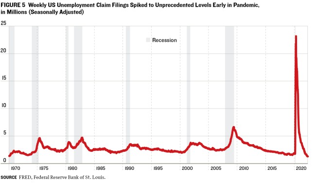
The global COVID-19 pandemic triggered a series of policy and economic shifts that posed unprecedented challenges for state budget forecasters. As the pandemic spread across the US in 2020, widespread shutdowns reduced economic activity, leading to over 20 million layoffs nationwide within two months.1 In reaction to this economic freefall, Congress initially passed a $1.7 trillion fiscal stimulus bill,2 while the Federal Reserve adopted expansionary monetary policy, cutting interest rates and stepping up bond purchases.3 As the pandemic unfolded, additional stimulus enacted by Congress pushed the total pandemic fiscal injection to more than $5 trillion.4 The influx of federal aid and the easing of shutdown policies, resulted in an economic recovery that began in May 2020. This recovery was followed by the highest inflation in decades beginning in 2021 and continuing into 2022.5
These trends drove state budget forecasts, which assumed continued growth in early 2020—before the pandemic—then changed to projections of economic collapse. Reopenings and stimulus measures caused forecasts to change again, to rapid growth and inflation. Forecasts are always inaccurate to some degree, but particularly so when economic changes occur quickly. When officials enacted state budgets for fiscal 2020 in the spring of 2019, it would have been impossible to forecast the early pandemic declines, which were unlike anything seen in nearly a century. Likewise, in March 2020, as pandemic-related shutdowns hit the economy, it would have been irresponsible for them to forecast a fiscal 2022 budget reflecting an overheated economy and inflation at forty-year highs. Yet that is what happened.
According to the National Association of State Budget Officers (NASBO), only six states had fiscal 2020 revenue collections that were close enough to the initial forecast to be deemed on target by state officials (figure 1). Thirty-five states initially overestimated revenue, basing their forecasts on economic and public policy responses to COVID-19, including a delay in collecting income tax.
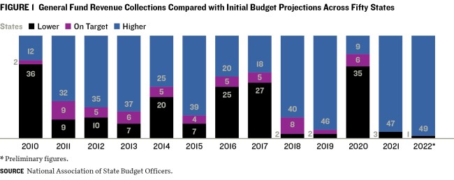
In fiscal 2021, during a strong recovery, no initial revenue projections were deemed on target; forty-seven states underestimated revenues (figure 1).6 Revenue over- and underestimates can undermine long-term budget stability. Overestimates may impair service delivery and prompt policymakers to focus on cutting an imbalanced budget every year rather than proactive future planning. In contrast, continuous underestimates may drive officials to underallocate resources, potentially disrupting critical public services.
Fortunately, state budget processes are iterative. Forecasts should change when conditions do. Even so, forecasts must work in concert with other budget tools to ensure long-term fiscal balance. Such tools include control of the revenue system, an ample range of budget reserves (including and in addition to formal rainy day funds), cash flow management, and agency spending adjustments.
For purposes of this paper, budget forecasting means establishing a point forecast, or specific dollar amount, used to balance a budget. Some states also conduct scenario planning, which considers a range of possible outcomes based on historical trends. In setting the point forecast, officials may consider both the range of potential estimates and the strength or weakness of other budget mechanisms. (These valuable approaches inform, but differ from, the budget point forecast itself because a budget cannot be balanced to a range estimate.)
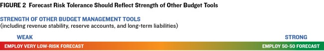
The various budget tools should be deployed regularly in conjunction with one another. For example, to maintain structural budget balance, a state that is highly reliant on volatile revenue sources, has depleted its rainy day funds, and is not fully funding long-term liabilities such as public worker pensions, mayday funds, and is not fully funding long-term liabilities such as public worker pensions, may need to hedge against these shortcomings by using a low-risk forecast, such as one with a 90 percent or greater probability of meeting the target. But a state with more stable revenues, ample budget reserves, and low long-term liabilities may have the fiscal flexibility to employ an unbiased, fifty-fifty forecast (figure 2). This is an estimate with equal upside and downside risk of not being realized.
FORECASTS SHAPE THE BUDGET PROCESS
Building the Foundation
Forecasts underpin the state budget process by establishing key assumptions used to prioritize budget allocations. A forecast of growing revenue signals opportunities for spending or tax cuts, while a declining-revenue forecast signals expenditure cuts or tax increases to maintain budgetary balance. These stakes may tempt policymakers to skew budget forecasts toward their preferred spending or tax outcome. But inaccurate forecasts focused on the short term may create future problems. Long-term fiscal sustainability and reliable service delivery depend on reasonably accurate budget forecasts.
To facilitate meaningful public participation and encourage long-term budget thinking, the Volcker Alliance recommends that states adopt and articulate four process-related forecasting practices in budget and planning documents:
- Consensus executive and legislative branch revenue estimates
- Reasonable and detailed rationale supporting revenue projections
- Multiyear revenue forecasts spanning at least three full fiscal years
- Multiyear spending forecasts spanning at least three full fiscal years7
Even with these practices in place and normal economic times prevailing, state budget forecasts are never exactly accurate because they must account for so much that is unknown. Economic disruption dramatically exacerbates this uncertainty, as the COVID-19 pandemic highlighted. Moreover, forecasts become increasingly speculative the longer the time horizon extends. Yet even with forecasts' inherent flaws, good forecasting practices and long-term scenario planning can inform and reinforce a commitment to long-term structural budget balance and can help with other budget decisions, such as setting aside adequate reserves or appropriately allocating funds between ongoing commitments and one-time projects based on revenue stream reliability.
Whether made in normal or highly precarious times, every budget design decision—including how aggressively to forecast state revenue and spending—entails an opportunity cost that budget makers often feel keenly. Opportunity costs may include withholding funding for a budget request for critical services or imposing tax levels that cause economic damage that outweighs projected benefits. Reasonable forecasts are essential to a sustainable budget process. Sudden program cuts (for instance, to courts, public safety, transportation, social services, or education) or tax increases to deal with a short-term cyclical gap may have a more devastating impact on the lives of state residents than actions based primarily on long-term strategic thinking.
Forecasts Are Imperfect
One truism about budgeting is that the forecast will always be wrong. It’s just a question of how wrong. Income tax revenues may come in above forecast. Fuel taxes may trail expectations. Medicaid may enroll fewer recipients. Judges may sentence more offenders to prison than projected. A recession may reduce revenues and prompt laid-off workers to pursue higher education, inflating state university costs and budget requests. A congressional budget impasse may delay or reduce federal funds.
Budgeting would be a simple exercise if policymakers knew the exact short-term and long-term outcome of every revenue and spending decision in advance. But this theoretical ideal isn’t reality. A forward-looking budget forecast can only roughly approximate the future. Forecasters must estimate future state revenues and costs sensibly with the estimates, based on past and present data. They must consider major cost drivers like school enrollment, Medicaid caseloads, and changes in the prison population. Forecasts also factor in economic variables such as inflation, business production, and household consumption, and the potential impacts of past and future fiscal policy decisions. For example, to reflect these uncertainties, the California Legislative Analyst’s Office regularly presents a range of possible long-term budgetary outcomes (figures 3 and 4).
Why Forecasts Differ: The Scientific Art of Forecasting
State forecasts nearly always involve mathematically exploring relationships between economic variables and state revenues by using statistical analysis methods such as regressions. Projections differ when forecasters use different economic variables to develop statistical models. Even forecasters anticipating the same economic variables may reach different conclusions, depending on the projection method used and period selected. State budget forecasts blend data science with professional judgment. They combine regression equations using the most salient economic variables with insights from business leaders about real-time experiences, forecasters’ gut feelings based on previous examples, and unstated or explicit hedges against potential negative outcomes.
CASE STUDY: California’s Legislative Analyst’s Office Uses Long- Term Forecasts and Portrays Forecast Uncertainty
California provides a case study in the use of long-term forecasts that portray greater uncertainty in future years. The Volcker Alliance gave the state a B average grade (the second-highest mark) in budget forecasting for fiscal 2015–19, partly for its use of multiyear revenue, expenditure, and economic forecasts. California did not to receive the highest grade because it does not use a consensus forecast process that includes estimates from the executive and legislative branches.8
In addition to developing point forecasts used for budget balancing, the Legislative Analyst’s Office (LAO) has worked in recent years to directly convey forecast uncertainty. Addressing a range of potential revenue forecast risks helps legislators make informed decisions about the consequences of their enacted budget, as they can select their risk tolerance level as a matter of enacted policy rather than through a staff decesion behind-the-scenes.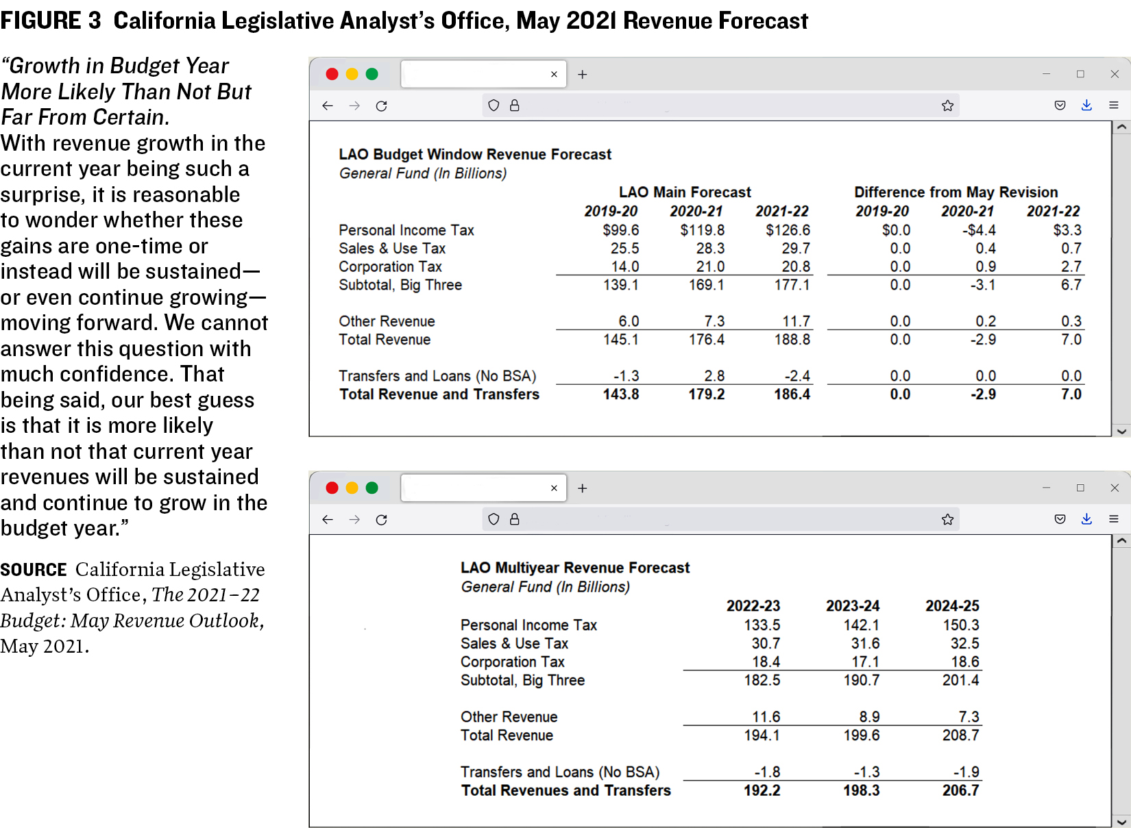
Figure 3 shows the LAO's May 2021 Main Forecast for the general fund for the budget window (the period over which officials balance the budget) and contrasts it with the governor’s 2021 May Revision forecast. While the legislative and executive branch forecasts differ because the state does not use a consensus process, the two are in close alignment for the then-current year (fiscal 2020–21) and budget year (fiscal 2021–22). In addition, the LAO forecast includes the office’s long-term estimates, which cover three years beyond the budget window.
Figure 4 provides two examples from different documents that communicate this uncertainty. The LAO derives the illustrated range boundaries from historical highs and lows over the business cycle.
In an interview for this paper, California Legislative Analyst Gabriel Petek said, “The purpose of highlighting a range of potential economic outcomes based on historical performance is to engage in dialogue with the legislature about its collective risk tolerance level. A riskier forecast may allow higher spending, but at the risk of having to come back later and cut spending. A very low-risk forecast may avoid the downside risk of later cuts but misses out on opportunities
to productively use scarce state resources.”9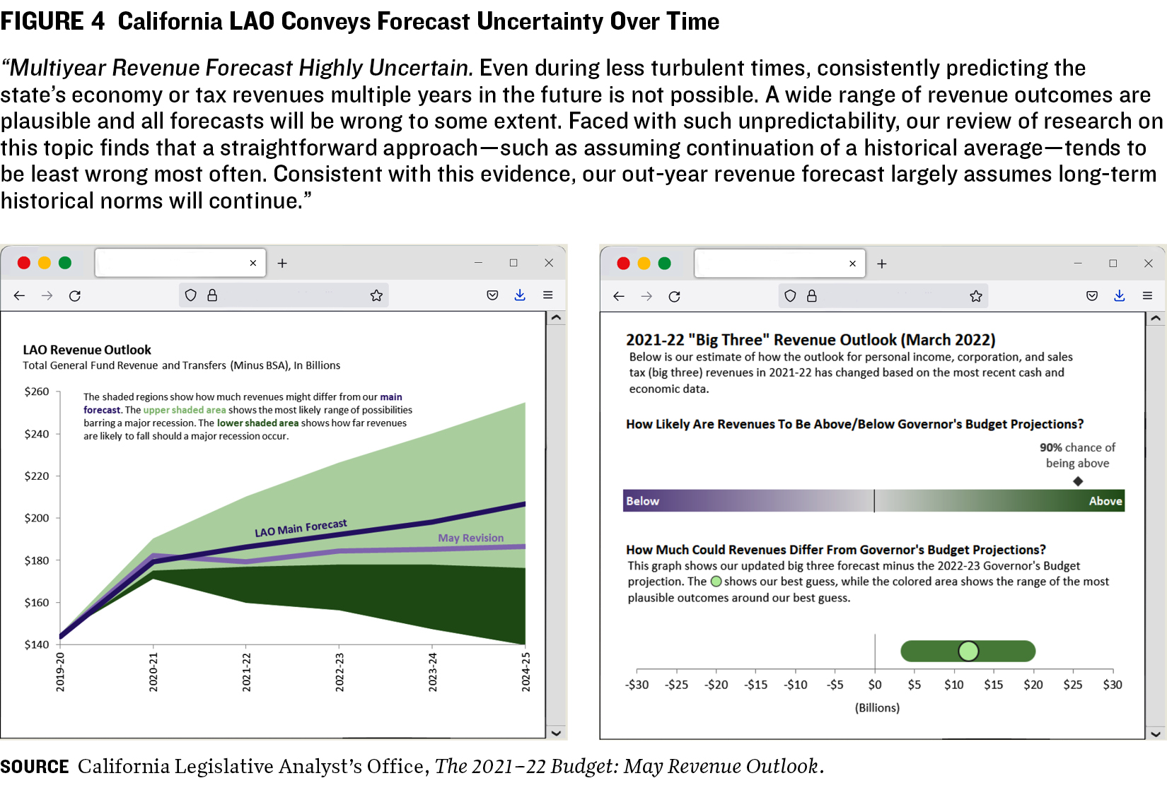
The initial LAO revenue outlook in figure 4 shows a narrow general fund collection range for the current year (fiscal 2020–21) because the forecast incorporates actual data for the first ten months. Uncertainty increases dramatically in each successive year. Potential revenue for the budget year (fiscal 2021–22) ranges from about $160 billion to $210 billion, with the LAO’s main forecast centered between the high and low figures. Given the economic cloudiness in the pandemic’s aftermath, note the even wider range by fiscal 2024–25: from about $140 billion, assuming a major recession, to about $250 billion, with strong economic growth.
Nearly a year after that forecast, the LAO’s 2021–22 outlook for personal income, corporate, and sales tax revenue—the so-called Big Three—showed a 90 percent probability that the governor’s revenue projection would be met. This means the budget was highly likely to result in a year-end revenue surplus. If, therefore, the legislature had been willing to assume more risk to get closer to a fifty-fifty forecast, it could have budgeted for moderately higher revenues.
FORECASTING AMID ECONOMIC CHAOS
The COVID-19 Effect
Predicting human behavior is a difficult task in the best of times, and more so in a volatile environment.
Forecasts made amid economic chaos can be very wrong, as the Congressional Budget Office (CBO) discovered in the Great Recession of 2007–09. Congress authorized $700 billion for the federal Troubled Asset Relief Program (TARP), an effort to support key industries. Aid recipients provided certain assets as loan repayment guarantees. The CBO initially estimated that the net program cost after asset sales would total $356 billion over its standard ten-year forecast period.10 As TARP wound down a decade later, the CBO estimated the net cost at $31 billion—less than a tenth of the original sum—because the economic recovery supported higher-than-projected collateral values.11 In this case, highly credible forecasters were off by an order of magnitude on their cost estimate of one of the highest-profile bills enacted to combat the recession.
COVID-19 also provided daunting fiscal forecasting challenges. When policy responses to the COVID-19 pandemic curtailed substantial portions of US economic activity in 2020, states revised budget forecasts repeatedly to incorporate new information. Many states swung from original projections of underperforming revenues in 2020, which required budget-balancing actions, to dramatically outperforming revenues when shutdowns eased and federal aid flowed in 2021 and 2022.
For federal fiscal 2021, the CBO’s error—the difference between the actual value and the estimate—in the March 2020 forecast was a 15 percent underestimate for revenues and a 4 percent overestimate for spending. This was two to three times the office’s average absolute error of 5 percent and 2 percent, respectively, in its forecasts over decades.12
Similar to federal forecasting difficulties, governors’ state budget recommendations released in December 2019 and January 2020 (before the pandemic in the US), initially projected solid increases of nearly 3.5 percent in general fund revenues for fiscal 2021.13 Amid the longest sustained period of economic growth on record,14 unemployment was expected to remain low.15
This changed dramatically with the pandemic. Figure 5 shows initial US unemployment claims, which rose to historic levels at the end of the first quarter of 2020. As shutdowns and fear gripped the country, other economic data also signaled a severe downturn. State forecasters revised their revenue forecasts in real time, without having a clear understanding of the pandemic’s path, duration, or how public health policies would affect the economy or revenues.
As the pandemic spread, enacted fiscal 2021 budgets (generally for the fiscal year beginning July 1, 2020), dropped a total of about 5.5 percent from governors’ initial recommendations. Budget timelines vary, however, so states enacted budgets at different points during the pandemic. Some states with biennial budgets did not adopt a new budget in 2020, while others with annual budgets enacted plans in May and June 2020 that projected year-over-year revenue declines of 20 percent or more.16 These extreme forecasts were based on early economic indicators that dwarfed those of previous recessions, including the 2007–09 downturn, and
on the federal government’s unprecedented adjustment to its deadline for filing income tax.
Shortly after the public health crisis began, the federal government enacted the first of three waves of pandemic-related funding (figure 6). From March 2020 to March 2021, Congress passed a series of fiscal stimulus bills, equivalent to nearly 25 percent of US gross domestic product. State budgets benefited immediately from direct state aid allocations and the indirect effects on state revenues of providing funds to keep households and businesses afloat.17 As a result, state forecasts turned from budget reductions to stability to increases.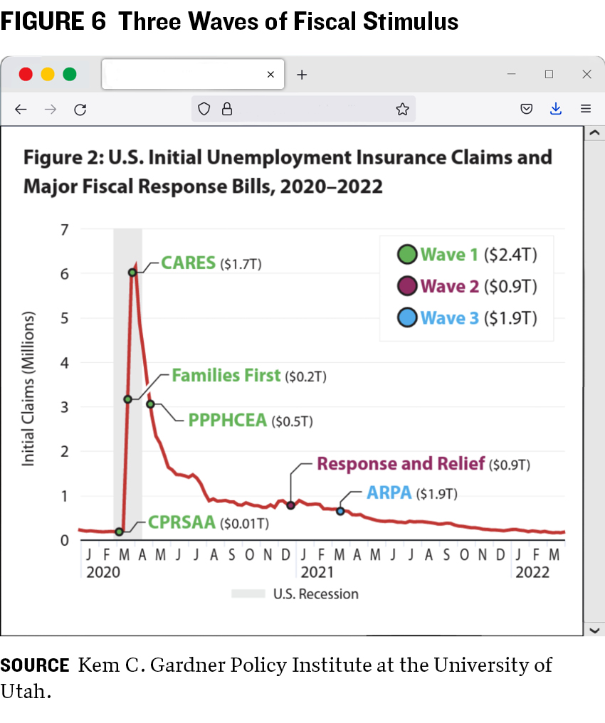
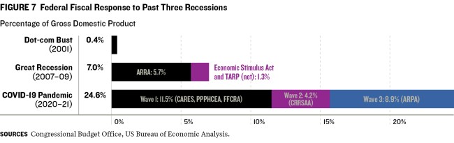
The size of the federal stimulus, some of it spread over several years, far exceeded the government’s fiscal response to recessions of the past two decades (figure 7) and dramatically altered the pandemic’s economic effects. After propping up an economy in freefall early in the pandemic, these historic fiscal responses also contributed to economic challenges as of this writing, which include goods shortages and inflation, and to state budget uncertainty. Since this level of fiscal stimulus had never occurred before, its economic effects remain unclear, making forecasts challenging. Officials in most states continue to wonder how much of the recent strong revenue collection is sustainable and how much is a sugar high resulting from federal fiscal and monetary stimulus.
States Employed Many Budgetary Tools as Pandemic Forecasts Changed
The pandemic led states to change budget forecasts and triggered the deployment of many other budget tools. These included using formal rainy day funds, borrowing internally, tapping restricted accounts, and cutting spending. Early on, the federal government delayed its date for 2020 income tax from April
15 to July 15. The majority of states that impose income taxes also delayed state filing dates to July 15. For states with annual budgets, this shift moved a sizable amount of revenue from fiscal 2020, which ends June 30 for most states, to fiscal 2021. For example, the shift reduced Utah’s fiscal 2020 income tax revenues by nearly $800 million, or about 17 percent, throwing that year’s budget out of balance.18 Forecasts ultimately assumed most of the revenue would be collected in July, but Utah and other states had to focus on managing an unexpected three month cash flow challenge.
In a series of interviews conducted for this paper, Utah and Maryland budget officials said they usually do not have to consider cash flow problems, thanks to healthy reserve balances. In the pandemic’s early turmoil, however, they faced unattractive options to raise needed cash, including potentially liquidating longer-term securities at fire-sale prices. Ultimately, the Coronavirus Aid, Relief, and Economic Security (CARES) Act facilitated cash flow through economic support to firms and households, along with $150 billion in Coronavirus Relief Fund emergency aid to state, local, tribal, and territorial governments.19 In Utah, to further support cash flow, the state piggybacked on federal aid by issuing general obligation bonds under a plan previously developed as part of its budget stress-testing process (see Utah case studies).
In California, budget officials borrowed internally early in the pandemic, leveraging restricted-account loans to balance the budget with state funds. In the years before the pandemic, officials had focused on repaying similar loans taken out during the Great Recession. In our interviews, executive and legislative branch officials reported that these repayments enabled them to borrow internally again during the COVID-19 crisis. Meanwhile, in Idaho, officials focused on strengthening the state’s long-term budgetary management tools (see Idaho case study).
CASE STUDY: How Utah Used Restricted-Account Reserves and the Capital Budget as Buffers
Utah went into the pandemic with its budget forecasting process already fortified. While the state earned a B average from the Volcker Alliance in budget forecasting for fiscal 2015–19, it garnered annual A grades in 2018–19 after enacting a statute in 2018 that directed the Office of the Legislative Fiscal Analyst to make long-term revenue and expenditure projections for major tax sources under different economic scenarios as part of a budget stress-testing process.20
Utah was already using consensus revenue and spending estimates produced jointly by the executive and legislative branches and disclosed its economic projections.
Utah drew down budget reserves to make up for the forecast fiscal 2020 revenue declines—a result of slowing economic activity and moving the income tax due date. Forecasts indicated that the state would collect the delayed income tax in July 2020 (after Utah’s July 1 start date for fiscal 2021). Utah’s nearly $800 million budget adjustment required to offset the delay in income tax was made primarily through internal borrowing from restricted-account balances. The state repaid this internal borrowing in fiscal 2021, when it collected the taxes. Notably, it did not need to draw on its formal rainy day funds. Rather, Utah used other budgetary reserves, which typically tend to receive much less attention because they require deeper knowledge of a state’s budget.
During periods of economic growth, Utah budgets ongoing general fund and restricted account revenues for new, one-time capital expenditures, such as for buildings or roads. These “working rainy day funds,” in Utah budget parlance, constitute a key relief valve. Unlike a normal rainy day fund, these funds do not sit in a bank but circulate into the economy via capital projects. Importantly, they do not pay for ongoing maintenance, which has another funding source. During economic downturns, the state can choose to either delay new construction projects or issue bonds for them. Through this mechanism, Utah can free up some or all of the ongoing funds previously allocated to one-time projects. These funds can then be shifted to cover revenue losses, thereby shoring up funding for programs such as education or Medicaid, the joint state and federal health care program for lower-income residents.
For example, Utah recently moved its primary state prison from a dilapidated 1950s-era facility in the Silicon Slopes area, about twenty miles south of Salt Lake City, to a new complex near the Great Salt Lake. In addition to financing the $1 billion project with one-time revenues and bonds, the state allocated $110 million of ongoing revenue for construction. That is, Utah set aside $110 million of recurring funding for a project of limited duration. Had a downturn not occurred, that same amount of ongoing spending capacity would have been freed up on completion of construction, as it was a one-time project. This would have created a structural budget surplus. But the pandemic hit before completion. By early April 2020, Utah had pivoted to issuing bonds for the prison rather than paying cash for the remainder of the project. While a portion of the $110 million in ongoing funds covered bond debt service expenses, this budget action freed up funds beyond those needed for the debt service payments. This approach helped manage both cash flow and the budgetary impacts of the early pandemic.
CASE STUDY: How Idaho Focused on Long-Term Management
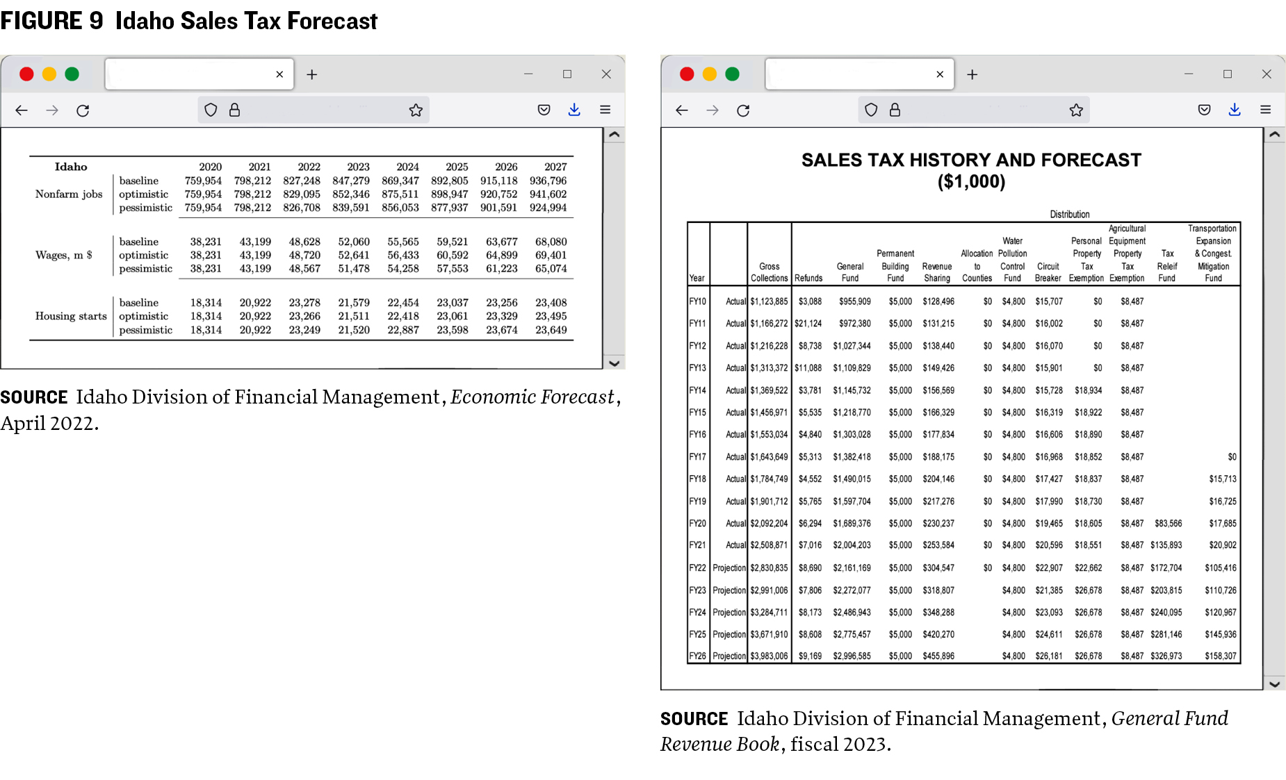
The Volcker Alliance assigned Idaho a D average grade—the lowest possible mark—in budget forecasting for fiscal 2015–19, largely because of its lack of a consensus revenue forecasting process and reliance on estimates for revenues and expenditures only for the upcoming fiscal year.21 During the pandemic, however, the state bolstered its longterm budget management focus. Under Governor Brad Little’s Executive Order 2021–10,22 the state adopted five-year budgetary forecasts, budget stress testing, and defining and addressing the cost of deferred infrastructure maintenance (figure 9).
Weathering the pandemic meant rethinking how Idaho forecasts revenue and expenditures, according to Alex Adams, administrator of Idaho’s Division of Financial Management. “We adopted five-year forecasts for both revenue and expenditures and leveraged alternate scenarios to account for different economic situations that may materialize,” he said. “This helped us think through the range of options available,” he added. “If revenue does not meet projections, [then it] gave us comfort that we can deliver on our obligation to have a long-term structurally balanced budget.”23
EIGHT BUDGETARY LESSONS FROM THE PANDEMIC
The COVID-19 pandemic highlighted ever-present challenges to state budget forecasting. The dramatic consequences of a worldwide pandemic were far from forecasters’ minds in the spring of 2019, when state budget officials projected fiscal 2020 revenues and expenditures. Federal government and Wall Street forecasters were hardly different. None knew that the next year would bring widespread economic damage as the government responses to the COVID-19 pandemic substantially shut down portions of the economy.
Similarly, early in the pandemic, in March and April 2020, it was hard to imagine budgeting for what was soon to be the situation: an overheated economy with high inflation, labor shortages, and extremely strong tax revenue growth. Fortunately, states aren’t tied to their original estimates, which they regularly update at different points in the budget cycle. In fact, the entire budget process, including forecasting, is an iterative process in which adjustments and corrections are made regularly.
The whipsaw nature of the pandemic highlighted both forecasting challenges and the need to prepare during good times for sudden fiscal tumult. Although the fine details of planning often go out the window when the unexpected happens, such crises highlight the value of establishing reserves and other budget tools during calmer times. As one California budget official told us, “You’ve got to repair the roof while the sun is shining.” Following are eight key lessons derived from research for this paper, including discussions with executive or legislative branch state budget officials in Alaska, California, Connecticut, Idaho, Maryland, and Utah. The six provide a sampling of large and small states with varied economic and fiscal profiles.
1. Budget Resiliency Matters More than Precise Forecasting
Every state budget official interviewed noted that forecasts will inevitably be wrong and require periodic updating. Unexpected events can quickly make forecasts or other budget plans obsolete. Options for fiscal responses to a downturn—whatever its specific origin—help with quick execution of budget actions during economic upheaval. While none of the officials projected the pandemic in early 2019, they generically considered preparing for future downturns as they made budget decisions. Budget officials from all six states studied said they were glad they had done important fiscal work in prior year, including maintaining or moving toward structural balance, building rainy day funds and other budget reserves, scenario planning through budget stress testing,and preserving borrowing capacity. Fiscal preparation proved key to navigating a black swan event like the pandemic.
2. Timing Is Everything
Several state officials said that it may be appropriate to let normal budget processes work during a crisis, rather than change course too quickly. The pandemic’s worst impacts occurred at varying points in budget cycles, so states reacted based on the best information available at the time of budget adoption.
Over- and under-correction can create budget challenges that may take years to resolve. If states wait too long to respond to a downturn, as some states did during the Great Recession, spending cuts become harder to implement, as more funds have been spent or contractually committed. Future reductions become deeper and more intractable.
But responding too quickly with deep budget cuts can lead to other challenges. For example, rash layoffs or incentives for early retirement as the pandemic hit would have exacerbated the labor shortages that emerged as the COVID-19 crisis ebbed and federal aid flowed. In the current tight hiring environment, it could take many years to replace an experienced employee’s institutional knowledge, impairing service delivery.
In Connecticut, which the Volcker Alliance awarded an A average grade in budget forecasting for fiscal 2015–19,24 officials indicated that they probably would have overcorrected if, early in the pandemic, they had been at the beginning of their biennial budget cycle. Their standard budget process allowed time to see what developed before they reacted.
In California, which uses annual budgets, officials also said it paid off to let their process follow the normal schedule rather than overcorrect based on early projections of the pandemic’s impact.
3. Though Critical, Early Federal Support Created Issues
State budgeters said rapid early fiscal support from the US government was vital and justified, given the pandemic’s unprecedented impact and federal guidance to shut down portions of the economy.
In Maryland, which the Volcker Alliance awarded an A average in budget forecasting for fiscal 2015–19),25 officials acknowledged that because federal COVID-19 support put a floor under the economy, it paid to wait and see what the US was going to do as state officials made major fiscal decisions. States’ fiscal trajectory improved dramatically when Congress passed the first wave of pandemic spending and direct state aid arrived.
The Families First Coronavirus Response Act, enacted March 18, 2020, increased each state’s traditional Medicaid federal medical assistance percentage by 6.2 percentage points,retroactive to January 2020. Keely Bosler, who was director of the California Department of Finance during the pandemic, said in an interview for this paper that this boost provided immediate budget relief through an existing fiscal channel at a time when states expected Medicaid costs for new enrollees to increase and state revenues to decline as economic activity stalled.26
Yet federal actions during the pandemic came with sizable pitfalls for states. For instance, some of the 2020 CARES Act allocations to states came with year-end 2020 spending deadlines, yet formal guidance about how to leverage the funding came slowly and changed over time. In addition, the Internal Revenue Service’s decision to help taxpayers by delaying the 2020 federal income tax filing deadline to July 15 from the normal April 15 date did not take the budgetary impact on states into account.
State officials understood pandemic funds were one-time allocations. States risked the burden of structural deficits if they used the one-time cash for recurring expenditures. As of 2022, many states continue to contemplate how to fully budget their share of $195.3 billion in State and Local Fiscal Recovery Funds provided by the American Rescue Plan Act (ARPA). For states that choose to spend the one-time money on ongoing programs, fiscal cliffs loom when the federal funds run out (2026 at the latest under current law).27 States must also deal with the surge in inflation tied to the fiscal and monetary stimulus and the effects of higher general fund expenditures driven in part by increased prices to deliver goods and services.
4. Prudent Spending Takes Time
Spending massive amounts of money sensibly takes time. Government procurement operations are designed to be deliberative. The CARES Act had extremely short spending deadlines (nine months after enactment) that led to some suboptimal outcomes as states rushed to spend money at a time of supply chain disruptions. Though state officials said they would change certain actions based on what they know now, they had to develop spending plans based on the best information available at the time. As that changed, so did their budgets.
5. Cash Flow Counts
Maryland and Utah officials expressed concerns early in the pandemic about cash flow, which had not been an issue in many years thanks to the states’ robust reserves. In addition to general economic declines, the change in the 2020 date for income tax filing, from April 15 to July 15, delayed collection of a significant amount of taxes, which added to cash flow uncertainty. The federal fiscal response, particularly the CARES Act enacted at the end of March 2020, alleviated cash flow concerns by providing aid to states and propping up the economy.
6. Formal Budget Reserves Are There for a Reason
Several state officials, including those from Maryland and Utah, commented on the reluctance some state policymakers have had to tap rainy day funds, both during the pandemic and previous recessions. Marc Nicole, deputy secretary of the Maryland Department of Budget and Management, said it’s important not only to think about sizing rainy day funds at the right level but also to be willing to use them when needed.28
7. Build Staff Capacity
Well-trained staff is critical to managing unexpected events. Some states hired new employees to handle the influx in federal funding, while others diverted existing staff. Building a workforce with competent, skilled employees in good times is critical to being prepared for a crisis.
8. For Every Budget Job, There’s the Right Set of Budget Tools
The pandemic highlighted the importance of making the best forecasts given available data, while simultaneously preparing for inevitable changes to these estimates. Budget responses to the global crisis (see Alaska case study) show that states can effectively leverage a broad array of budget management tools in concert with forecasts. Readily identified for all states, formal rainy day funds (or budget reserve accounts) may be the most visible budget tool to smooth out missed forecasts. These are other important tools:
- State revenue system design, including policy control of the tax base and tax rates
- Budget reserves, including one-time reserves other than formal rainy day funds—for example, unspent balances in the general fund and restricted or special funds whose use is legally prescribed—and working rainy day fund budget reserves in the form of ongoing revenues allocated to one-time projects. These include capital projects that can be delayed or funded with bond issuance during a downturn, freeing up ongoing funds for redeployment
- Cash flow management, including spending some revenues in the year or years after revenue receipt or shifting the timing of state payments
- Control of state agency spending for both the current year and future years, including through targeted or across-the-board budget cuts via program changes; personnel actions such as hiring freezes, furloughs, or layoffs; and local aid adjustments.
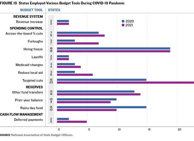
Figure 10 illustrates how states used many of these tools early in the pandemic. NASBO data show the breadth of options budgeters took, including various actions to control state spending. The data also show that fifteen states accessed formal rainy day funds in the final months of fiscal 2020, when other tools were more limited during the short time frame to respond. In fiscal 2021,fourteen states relied on borrowing or shifting funds from various special or restricted accounts, while ten accessed their official rainy day funds.
CASE STUDY: Forecasting Alaska’s Volatile Revenue Is Problematic, Requires Reliance on Other Management Tools
Alaska's budget process illustrates the interrelationship between forecasts and other budgetary tools, including revenue system design and reserve maintenance. The Volcker Alliance assigned Alaska an average grade of B in budget forecasting for fiscal 2015–19 for its use of ten-year revenue, spending, and economic forecasts. The state did not use consensus forecasts.29
The state economy depends on natural resource extraction, primarily petroleum. In 1976, the state created the Alaska Permanent Fund, a reserve totaling $80 billion intended to provide residents permanent benefits after natural resources are exhausted.30 According to state budget officials, Alaska’s unusual revenue design relies heavily on permanent fund investment returns and taxes on petroleum extraction industries. In fiscal 2023, these revenue sources provide over 90 percent of Alaska’s general fund revenue.31 Forecasters face major challenges accurately projecting these highly volatile revenue sources.
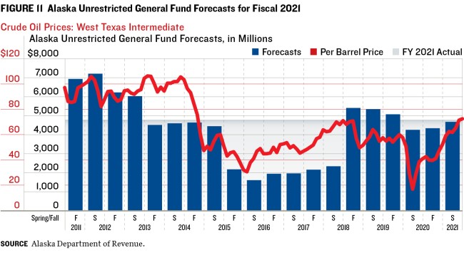
As shown in figure 11, Alaska’s short- and long-term revenue forecasts tend to follow crude oil prices, which can heavily influence state revenues. Early in the pandemic, petroleum prices fell nearly 70 percent as shutdowns suppressed consumer demand. Oil price increases, such as spikes as the pandemic ebbed, will now boost future revenue forecasts.
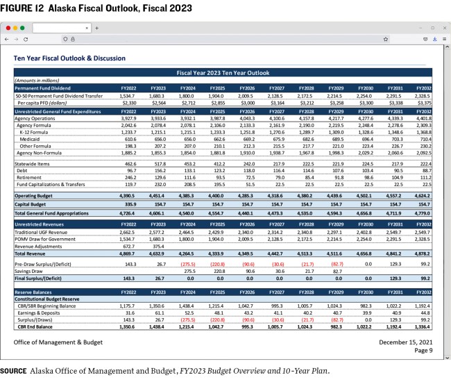
Because of its forecasting challenges, Alaska uses very long-term forecasts (figure 12). According to interviews with budget officials, the state has focused on maintaining large budget reserves when oil prices were high to offset the budget shortfalls that occur when oil prices drop. Alaska experienced a crisis in the late 1990s and early 2000s, when oil prices were low, and strengthened its long-term fiscal processes as a result. Higher oil prices in the mid-2000s temporarily abated the state’s fiscal challenges, but Alaska budget officials said the improvements proved their worth when oil prices dropped again in 2014.32
According to state officials, Alaska strives for transparency in revenue forecasts. The executive and legislative branches rely on the permanent fund’s investment adviser for a forecast of its returns, which make up about 60 percent of general fund revenues. Petroleum revenues make up 26 percent of general fund revenues.33 Because of time lags between forecast preparation and public release, Alaska shifted to using oil future market prices on a specified day to project revenues.
Because oil is a volatile revenue source, “we’ve always known we need to have a lot of reserves and to anticipate volatility,” Alaska’s legislative fiscal analyst, Alexei Painter, said in an interview for this report. “That means by our nature we need to do more long-term fiscal planning than most states.”
Since the large 2014 oil price decline, however, Alaska has consistently drawn down its sizable reserves. Before the recent surge in oil prices coming out of the pandemic, the state was in a precarious budget position, with an ongoing structural deficit and depleted reserves.34 To deal with these problems, Alaska could undertake a conservative revenue forecast with a high likelihood of being met. It could also focus on improving the status of its other budget tools, such as diversifying its revenue streams, adjusting state spending, and rebuilding reserves when oil prices increase—as they have recently—and recalibrate forecasts to that strengthened fiscal position.
How Alaska Deals with Volatile Oil Revenues
The following text is excerpted from the The Fiscal Year 2023 Budget: Legislative Fiscal Analyst’s Overview of the Governor’s Request, 2022, prepared by the Alaska Legislative Finance Division.
Forecasting Volatile Revenue
While Alaska‘s fiscal picture is much improved from a year ago, it is fair to ask whether the current higher oil prices will last. Alaska’s unique mix of volatile revenue from petroleum and investments makes predicting future revenue more difficult than in any other state. Investment revenue projections come from the State’s investment advisor, Callan and Associates. Oil revenue projections are developed by the Department of Revenue (DOR), with assistance from the Department of Natural Resources on the oil production forecast. Oil prices are the most impactful variable in forecasting petroleum revenues, and DOR has changed its methodology in recent years to improve accuracy and transparency.
How Should the Legislature Handle Volatile Revenue?
DOR’s oil price forecasting methodology is sound, but that does not mean that the forecast will come true—in DOR’s test, this method still had significant forecasting errors. Even the best-informed oil traders are not omniscient and cannot foresee technological breakthroughs, extreme events like the COVID-19 pandemic, or geopolitical developments. When the oil market is unsettled due to constantly changing events (such as the emergence of the Omicron variant in December 2021), oil prices and futures often change by several dollars per day. For example, the futures price as of December 5, 2021 would indicate an FY23 average price of $67.14, while the futures price three days later would indicate an FY23 price of $72.55. This $5.41 difference is worth nearly $322 million in oil revenue in FY23—enough to drastically change Alaska‘s fiscal situation. In the actual forecast, DOR smooths this in their forecast by averaging the futures market over five days, but the end result is still volatile. How can policymakers handle this volatility? Historically, Alaska has utilized our large budget reserves to smooth volatility from year to year—a $300 million budget gap could be filled from the Constitutional or Statutory budget reserves, or a windfall could help refill those reserves. Today, reserves have shrunk (the CBR had about $1 billion at the start of FY22 and the SBR was depleted), and the legislature failed to muster the supermajority votes to access the CBR in FY22 anyway. This means that in 2022 the legislature has fewer options to handle volatility than in years past.
CONCLUSION AND POLICY RECOMMENDATIONS
The pandemic showed the challenges state budget officials face in times of crisis, highlighting the need to integrate forecasts and other budget management tools. The unexpected economic disaster underscored key principles of best forecasting practices including:
- Forecasting matters. Though forecasts are inherently imperfect, without a forecast, budget balance cannot occur.
- Flexibility is vital. Closely monitor economic conditions. Forecast and reforecast to keep the budget in balance.
- Other budget tools are critical. State forecasts are one piece of the budget puzzle. States should consider revenue system design, informal and formal budget reserves, cash flow management, and spending control. The strength or weakness of these other budget tools should inform forecast risk.
- Scenario planning is necessary. Stress testing the budget by evaluating budget risks and reserves helps states determine areas to shore up and provides a blueprint for preparing for inevitable downturns.
- Consensus estimates and long-term thinking are needed. While no guarantee of forecast accuracy, consensus long-term revenue and spending estimates can help focus attention on long-term budget management.
- Forecasting includes future costs. States should evaluate their processes for reflecting fiscal impacts of new state legislative bills and allocate sufficient staff resources to properly estimate fiscal impacts of new bills.
Transparent assumptions are key. States should publicly articulate economic assumptions underlying budget forecasts. In addition, states should consider adopting these long-term budget management recommendations:
- Evaluate whether the baseline forecast approach is adequate given the state’s own revenue and spending volatility over the business cycle.
- Assess whether the state’s approach to estimating fiscal impacts for new bills is adequate, and allocate sufficient staff resources to do so if not.
- In public budget documents, specifically differentiate between one-time and ongoing revenues and spending.
- Conduct regular, formal scenario-planning exercises, possibly on a three- or five-year cycle, to assess the state’s budget resiliency against economic downturns, comparing value at risk and budget relief valves, to develop a downturn playbook prior to a crisis.
The pandemic highlighted at an extreme level the forecasting challenges states manage annually. Forecasts by nature are imperfect, so states must rely on a robust set of other fiscal tools to manage the inherent uncertainty. The time to build resiliency into these budget tools is when the economy and state revenues are strong, not during the time of crisis. Doing so can help states consistently deliver critical services to citizens during good and bad economic times.
APPENDIX: The Annual and Biennial Budget Process
In this appendix, we apply the lessons learned in A Cloudy Crystal Ball to create a set of best practices for executive and legislative officials to follow.
1. Budget Forecasting Nuts and Bolts
A. The Forecasting Process
Given forecast uncertainty and to allow for peer review from those inside and outside government, the Volcker Alliance encourages states to use a process for consensus revenue and spending forecasting between the executive and legislative branches and to clearly state the assumptions behind all forecasts.
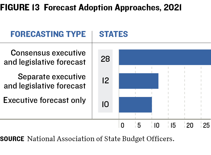
Formal forecast adoption processes vary among states, with twenty-eight using a consensus process, twelve using separate executive and legislative forecasts, and ten relying solely on an executive branch forecast (figure 13).
Under a consensus revenue forecasting process, the executive and legislative branches jointly arrive at the official state estimate. In some states, this involves a binding public process by a formal commission or similar group. In others, it occurs in behind-the-scenes discussions. The branches typically develop estimates
separately, then discuss and negotiate until they reach consensus. With a consensus forecast in place, both branches can work from the same set of basic revenue assumptions as they make budgetary changes.
This approach allows final budget talks to shift from debates over which revenue numbers to use to proactive planning. Through this process, extreme projections can be eliminated. While evidence that consensus forecasting improves accuracy is mixed,35 using such estimates can let officials benefit from the viewpoints and insights of numerous parties and potentially lead to more viable estimates and budget policy outcomes. The peer review inherent in a consensus estimate can provide a check against faulty budget assumptions. Maryland’s fiscal pandemic response highlights the benefits of a consensus forecast, particularly in times of economic stress. During the severe economic challenges in April 2020, the state comptroller (a consensus process participant) independently released a nonconsensus revenue estimate outside the normal process.36 Based on unemployment trends and shutdowns, the comptroller’s publicly available forecast indicated that 59 percent of sales taxes would be lost in the coming months. Actual monthly collections fell about 30 percent year over year,37 nowhere near as much as estimated by the independent forecast. A more robust peer-review process could have strengthened the comptroller’s forecast.
Despite their strengths, consensus forecasts have some drawbacks. For one, consensus budget estimates can inject highly politicized game theory into budget estimation, particularly in a formalized public process. Game theory involves how people behave in strategic situations and base their actions on others’ potential actions. Rather than focusing on technical interpretations of the economy and budget, forecast discussions can devolve into political grandstanding or manipulation. Additionally, while the executive and legislative branches sometimes have competing approaches, negotiating a consensus may involve agreements between politically aligned government branches that lead to a less accurate forecast. Consensus estimates can also mask uncertainty inherent in budget forecasting if people perceive consensus forecasts to be more accurate solely because participants agree to them.
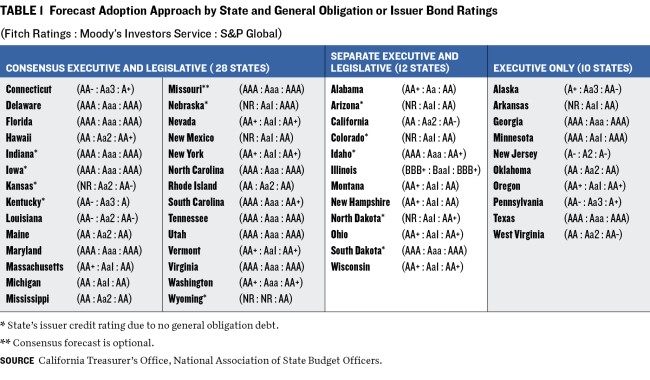
Of the sixteen states with an AAA general obligation bond or issuer rating from two or more of the three major rating agencies, ten use consensus forecasting; the remaining consensus states do not have a AAA rating from two or more agencies (See table 1). This suggests that rating agencies view consensus estimates not as a single predictor of bond repayment but as a practice that fits within the context of budget management practices. In addition, generally high state ratings (only Illinois is rated below A) suggest that agencies view those states as having a wide array of budget tools at their disposal to help secure bond repayment when forecasts miss the mark.
B. Forecast Timing
Budgeting, including forecasting, is an ongoing and iterative process. The first budget estimate is not the final word and can be updated to reflect the situation on the ground. As economic conditions alter revenue receipts or demand for certain services changes, policymakers have opportunities to update forecasts and revise budgets to incorporate these shifts. Such revisions may be made through formal actions, such as adopting new revenue or spending estimates, or through a governor’s administrative actions to constrain spending to match expected revenues.
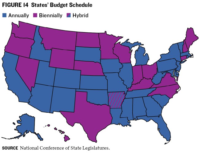
States forecast on different schedules based on their budget calendars. Elected officials in the executive and legislative branches and their respective appointed teams negotiate, adopt, and administer budgets over the state’s budget cycle, which is set in state constitutions and statutes. Thirty states budget annually and twenty budget biennially, or every two years (figure 14). The period over which states balance budgets is sometimes called the budget window; an out-year is a year beyond the budget window.
In most states, the governor releases budget recommendations between November and February—before legislative sessions begin. Legislatures then typically
adopt budgets for the following year (or biennium) from March through June. Forty-six states start their fiscal year July 1; four states do not, so their budget timing differs.38
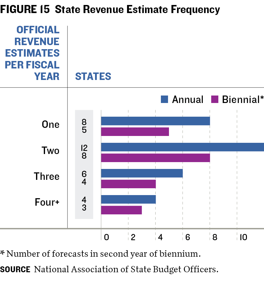
For both annual and biennial budget states, initial budgets typically use revenue estimates derived before the start of the fiscal year (late budgets may be an exception). This means that each budget cycle includes two or more forecasts—at least one preceding budget enactment and another during the budget period—allowing for midcourse corrections. Most states forecast even more frequently (figure 15), meaning that each budget will be subject to a series of estimates
to periodically fine-tune projections based on real-time conditions.
When conditions warrant, policymakers may alter adopted budgets midstream via supplemental budget increases or decreases. Spending reductions can often be accomplished through gubernatorial order. Legislative action may be required to enact cuts. If that is the case, part-time legislatures would have to convene a special session or adopt changes in the next general session.
C. Allocating Budget Office Staff Time
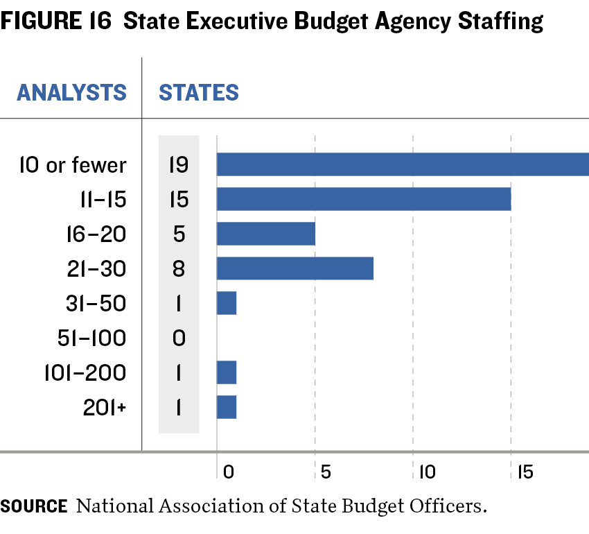
State budget offices face the real-world trade-offs of limited staff resources. According to NASBO, between fiscal 2008 (during the Great Recession) and fiscal 2021 (during the COVID-19 pandemic), the number of staffers in executive branch budget offices that were dedicated to the budget function fell by nearly 20 percent, from 1,764 to 1,433. While California and New York have large staffs, which account for about a third of this total, most states have much more limited staffing.39
Figure 16 summarizes analyst counts in state executive budget offices. Analysts are the largest component in budget staffing. As shown, nearly 70 percent of states scrutinize the revenue and spending sides of the budget with fifteen analysts or fewer. In building staff, budget directors must weigh the cost of assigning analysts to increase their understanding of state agency budgets against the incremental benefits of possibly more accurate economic and revenue forecasts. This enhanced staff knowledge can then be used to build resiliency into the budget itself.
Administering the vast federal funding increases that flowed through the states during the pandemic required staff. Some states hired new employees to administer the funding programs, while some diverted staff from other duties. The pandemic’s quick transition to remote work made it particularly difficult to hire and onboard staff, although this may be easier moving forward as hybrid work has become more commonplace. States should consider whether they have sufficient staff and expertise to manage budgets through the business cycle and, if not, develop plans to build that capacity over time.
D. Forecasting Tools
States generally use a combination of forecasts from national and state-specific data sources. Most use national economic forecasts from a diverse range of forecast providers, including the Congressional Budget Office, IHS Markit Global Insight, Moody’s Analytics, and Oxford Economics. Forecasters then augment these national forecasts with local economic intelligence from state agency, university, and private sector experts who may lend expertise in labor markets, real estate, natural resource production, technology, agriculture, and general business and economic conditions.
The Volcker Alliance recommends that states publicly articulate the economic assumptions that underlie their budget revenue and spending forecasts. Providing this information makes it easier to evaluate the reasonableness of budget assumptions. Common economic indicators used to forecast major state revenues include personal income, inflation, population
change, employment levels, and total and average wages.
State revenue and tax collection agencies often participate, formally or informally, in revenue projections, as they track real-time collections. Agencies managing major programs such as Medicaid, corrections and public safety, and education provide real-time insights
regarding state expenditure trends.
Forecasters meld national and state economic projections and actual year-to-date program costs and revenue collections into a unified budget forecast. They often rely heavily on econometric modeling, using data science techniques such as regressions and other tools to analyze how various economic indicators track with state revenues and spending.
This process can be challenging. Revenue collection or program enrollments, caseloads, and population trends sometimes vary from economic indicators. This variation can represent an early signal about pending economic changes, or it can be noise, explained by other factors. Economic models explore the relationships between indicators such as total wages, population growth, and state revenue collections and major program spending, such as Medicaid.
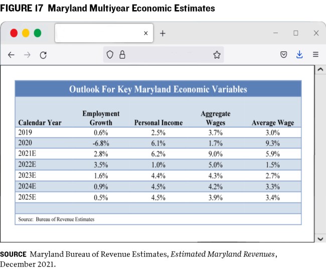
Complicating forecasts, these relationships do not remain constant but evolve with economic and state policy changes. For example, the relationship between total personal income and the sales and use tax base (total statewide taxable sales) has changed over decades. This occurred as household consumption shifted from goods, which are generally subject to sales taxes, to services, which often escape similar taxation. The rise of e-commerce further complicated sales and use tax forecasts, as uncollected sales and use taxes on purchases from out-of-state sellers altered the connection between household spending and sales and use taxes. This relationship shifted again in recent years as Amazon.com Inc. and other major online retailers began collecting and remitting sales taxes following to court decisions and legislative and administrative policy changes related to remote sales. Economic models attempt to capture the effects of these changes. (Figures 17 and 18 show examples from Maryland and California, which disclose their forecasts’ economic assumptions using multiyear estimates that extend beyond the budget window.)
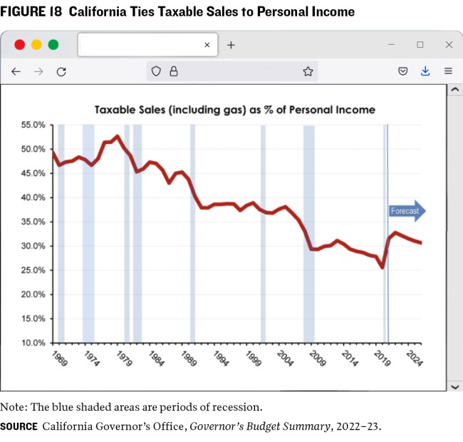
California’s Department of Finance illustrates the changing relationship, as taxable sales as a percentage of personal income declined by half over forty years—(from about 50 percent in the 1970s to about 25 percent in 2019) (figure 18). This decrease reversed for a few years as California collected more remote sales after the US Supreme Court’s 2018 South Dakota v. Wayfair, Inc. decision, which upheld that state's law requiring most out-of-state sellers to collect and remit sales taxes on goods and services delivered in the state. Most states have followed South Dakota’s example.40 During the pandemic, however, large-scale service shutdowns combined with federal fiscal stimulus moved consumption back toward taxable goods. As shown, California projects a gradual return toward prepandemic consumption behavior over time.
A forecaster may harness modern computational power to quickly run many simulations and employ hundreds of forecasting techniques, to establish lower and upper forecast bounds, incorporating historical trends, and then select the point forecast within that range of possibilities. One modeling tool that can help states think about uncertainty is a Monte Carlo simulation, which adds the element of forecast randomness to provide insight into the range of possibilities given certain historical parameters. While still new, machine learning tools can take this approach even further, as computers use historical data to set the parameters on their own.
Most budget estimates are not unbiased. That is, budget outcomes do not end up above and below the forecast in equal proportions, as occurs with a true fifty-fifty forecast. This occurs because many forecasters hedge their predictions. The immediate consequences of an upside risk—more money available than was projected—tend to be less dire than a downside risk. In other words, budget shortfalls often bring more undesirable consequences than surpluses. Downside-risk consequences include, at the extreme, massive layoffs and cuts to critical programs; milder consequences include use of reserves intended for another purpose or a confrontation between budget staff and an elected official upset about the political effects of a shortfall. Conversely, forecasters may also face political pressure to forecast revenues too ambitiously to temporarily “solve” a budget problem by pushing it into the next fiscal year.
Many state forecasters hedge at least slightly by underestimating revenues and overestimating spending. After all, when budget surpluses occur, money can be spent or returned to taxpayers a year later. But even the comparatively positive outcome of a budget surplus is not without consequence. Consistent revenue underestimates and expenditure overestimates that result in large surpluses year after year can lead residents and policymakers to believe taxes are too high—even if the surplus is primarily due to forecasting practices rather than excessive funding relative to legitimate service demands.
In addition, a consistent, sizable budget surplus can change which programs receive funding. Structural budget balance requires that spending not exceed revenues over the business cycle. This means one-time revenues, such as unbudgeted collections that exceed the forecast, should not continually fund ongoing expenses. These ongoing expenses are often people-oriented items, such as those funding employee pay, education, or social services. Common one-time spending categories such as buildings, roads, and equipment are objectoriented allocations (which should also benefit people indirectly). So the immediate effect of underforecasting revenue may be to shift funding from people-oriented programs toward object-oriented ones. Although ongoing revenue that could be allocated to people-oriented programs may show up in revenue forecasts the following year, those shifted one-time funds might not be allocated to the highest-priority need and thus may miss time-sensitive opportunities to improve lives.
To the extent that revenue over- or underestimates affect budget funds, the steps in the forecasting process constitute policy decisions in and of themselves. States sometimes establish this risk-management policy through the explicit and informed choices of elected officials. But sometimes it instead becomes a behind-the-scenes staff decision that elected officials do not explicitly make. With this level of forecast uncertainty, states should carefully consider their process for determining the level of forecast risk they are willing to tolerate.
2. What Do States Forecast?
Unlike the US Constitution, state constitutions generally require balanced budgets. More easily changeable state statutes, formal rules, and practices further develop budget processes within these constitutional contours. There’s disagreement about the exact definition of structural budget balance over time. But over the business cycle, most states cover annual state operating expenses with annual tax and fee revenues rather than incurring debt for recurring operating expenses, as the federal government does.
In general, states reserve bond issuance to cover long-term capital expenses. But some states seek to balance the budget over the short term by failing to fully fund such long-term liabilities as pensions and other postemployment benefits, including retiree health care. States should use long-term forecasts that fully incorporate these recurring costs into their budgets.
To determine budget balance, states formally adopt baseline forecasts for revenues and authorized spending. Executive and legislative budget offices typically give the most attention to the largest revenue and appropriation categories (the so-called Big Rock budget drivers), as these have the greatest ability to materially affect the overall budget.
-
BASELINE REVENUE FORECASTS Although state revenue sources vary, individual and corporate income taxes and general saes and use taxes constitute the two largest revenue sources for most states. Other sources include excise taxes such as those on cigarettes, and other tobacco products, natural resource severance taxes, and gaming revenue. Federal funds make up about a third of states' total budget revenues.41
-
BASELINE EXPENDITURE FORECASTS Spending forecasts generally focus on major enrollment-, caseload-, and population-driven programs such as K–12 and higher education, Medicaid, and corrections. As a joint federal-state entitlement program, Medicaid forecasts incorporate both funding components. K–12 funding forecasts often combine local property tax and state funding components.
State budgeting occurs in different funds. These can be thought of as checking or saving accounts set aside for specific purposes. Understanding the various funds is critical to understanding state budgeting, because each fund has its own budget discretion and forecast attention level. These are the fund types:
-
GENERAL FUND A state’s general fund is the most discretionary state fund that budget makers allocate. General fund revenues generally can be spent for any purpose. Given the wide policy latitude, general funds often generate the most intense competition for resources and scrutiny. Although budget parlance varies by state, the general fund is a fixed appropriation fund, meaning that the governor or legislature ensures that the fund appropriately balances revenue and spending. Therefore, governors, legislators, and their budget teams devote the greatest time and attention to general fund revenue and spending forecasts. In making budget allocations, states face trade-offs between a revenue-driven process, in which available revenues drive spending, and a spending-driven one, in which policymakers first scope out potential service needs, then design revenue systems to meet them. In practice, existing tax laws drive much of the budget process because voters tend to oppose tax increases. However, a spending-driven approach sometimes serves as the impetus for tax changes.
-
RESTRICTED OR SPECIAL FUNDS State accounts other than the general fund have revenue usage restrictions set by state constitution or statute. For example, states generally restrict or dedicate agency fees such as inspection, registration, or park entry charges to cover related service delivery costs. They occasionally assign certain taxes to a specific use, such as state fuel taxes for transportation expenses. Restricted funds are often called variable appropriation funds. This means that even if the legislature authorizes higher spending, state agencies collecting revenues through fees or other sources cannot spend more than actual revenues. Due to this feature, state agencies often forecast these accounts, subject to review by executive and legislative fiscal staff. But central budget offices may estimate and closely track large or politically sensitive restricted or dedicated revenue sources, such as fuel taxes. Moreover, these funds are sometimes redirected or borrowed against to cover general fund shortfalls.
-
FEDERAL FUNDS Federal funds are typically restricted to purposes authorized by the US government. For example, Medicaid is the largest federally funded program administered by states and represents roughly 60 percent of all nonpandemic federal funds flowing through state budgets.42 Because Medicaid requires that funds be used for certain health care services, states cannot apply that money to increasing teacher salaries or building roads. By projecting Medicaid expenses, state budget officials forecast the majority of standard federal funds in state budgets. Sometimes, as with Medicaid, states combine federal funds with state funds in restricted accounts to ensure that the money pays only for qualifying services. Other large federal allocations help pay for continuing social services programs, transportation, and K–12 education, which includes special education programs, high-poverty schools, and school lunches. In general, non-Medicaid federal funds tend to receive less forecast scrutiny, as they are generally considered variable funds, within which state agencies have to manage their spending if anticipated federal revenues do not materialize. During the last two recessions, the federal government allocated sizable amounts of discretionary state aid through the American Recovery and Reinvestment Act (2009), CARES Act (2020), and ARPA (2021). Unlike ongoing federal funds, these stimulus measures provided one-time revenue infusions that required states to take precautions to avoid creating future structural budget imbalances by devoting funding to ongoing programs.
-
TOTAL (ALL FUNDS) BUDGET The total or all funds budget comprises money from all funding sources described above, including the general fund, restricted state funds, federal funds, and even sometimes certain local funds, such as for education, incorporated into state funding formulas.
3. Forecasting for the Long Term
A. Cyclical and Structural Trends
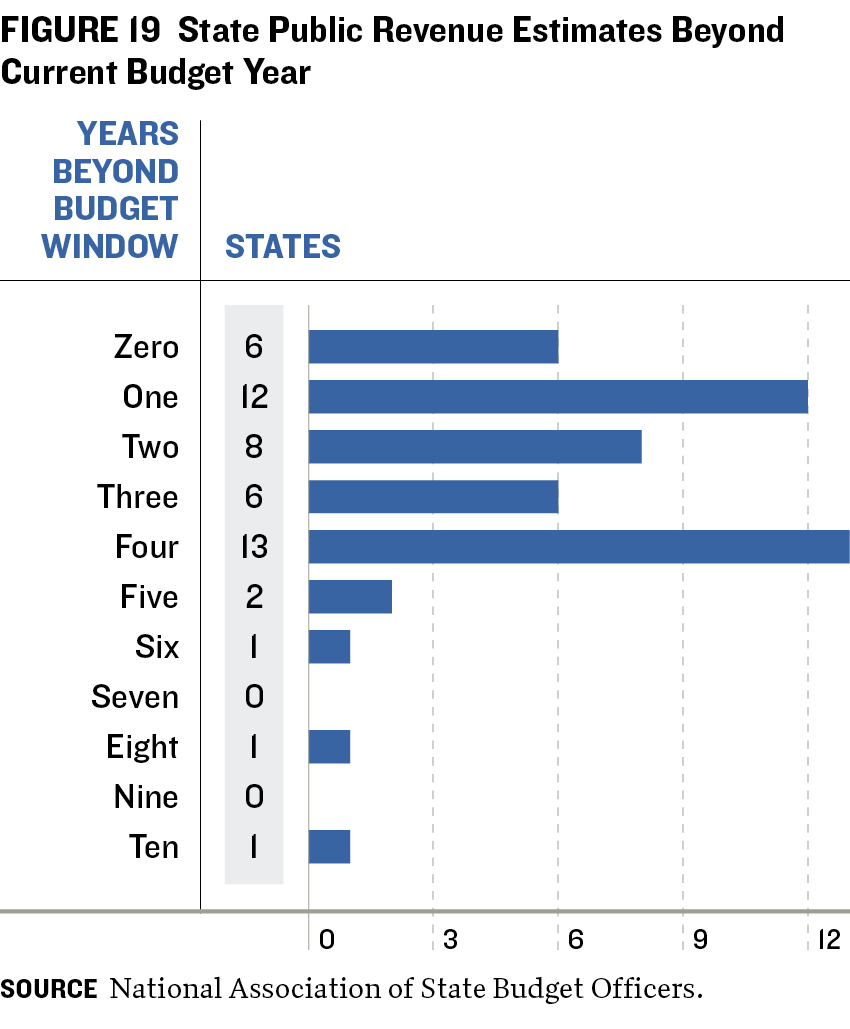
Forecasts based on the effects of current taxing and spending policy as well as those for adjusted taxing and spending policies should address short-term cyclical and long-term structural trends beyond the budget window (figure 19). A budget window is defined as the number of years over which the state balances its budget via adopted budget bills. A short-term cyclical trend may make budget savings appear to be available for long-term spending commitments. For example, a one-time income boost due to a federal tax change that artificially accelerates income realization in one fiscal year, but will be offset by less income in the following year, should not be considered ongoing revenue. The income boost should be offset with an offsetting one-time revenue reduction the following year. Similarly, states should consider longterm demographic and economic trends in long-term budget estimates.
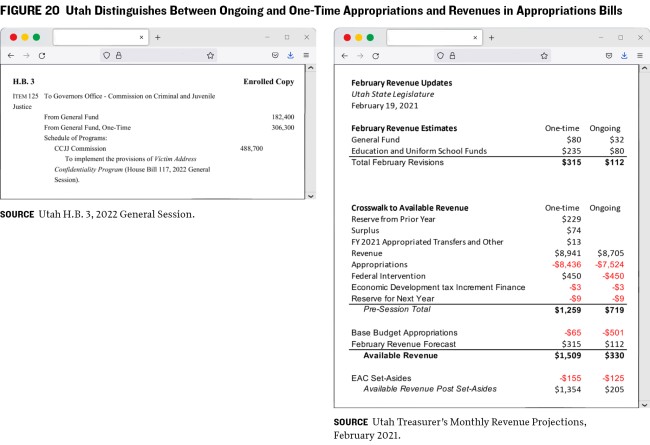
Prudently managing a budget means maintaining long-term structural balance. Structural balance means that ongoing state spending does not exceed ongoing revenues over the business cycle. Understanding structural balance requires distinguishing between one-time and ongoing revenues and spending (figure 20). One-time revenues (such as rainy day fund withdrawals during a recession or tax windfalls from a short-term federal tax change) should not regularly fund appropriations for ongoing programs. Conversely, appropriating ongoing revenues to one-time expenses like new facility construction can create a structural budget surplus that provides a fiscal cushion when the one-time project is completed.
Unfortunately, forecasters cannot easily identify all one-time general fund revenue increases or spending declines. Unlike recent one-time federal funding provided to states through CARES and ARPA, determining one-time and ongoing revenues from typical state sources requires thoughtful review. One-time revenue sources include legal settlements, year-end surpluses from the prior budget period, an increase in estimates for the current year, and state income-tax payment acceleration driven by changes in federal law.
A portion of excessive revenue growth out of line with long-term trends could also be a one-time source, but forecasts should consider the details of fundamental revenue structures rather than becoming too prescriptive based on historical trends. For example, to the extent revenue trends closely follow recent high inflation, a forecast of higher-than historical ongoing revenue growth may not necessarily be out of line if it reflects a structural economic change to inflated price levels.
B. One-Time versus Ongoing Revenue and Spending
Even though states set and administer budgets over a relatively short period, taking a longer-term budget perspective is critical to prudently managing the budget
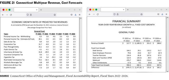
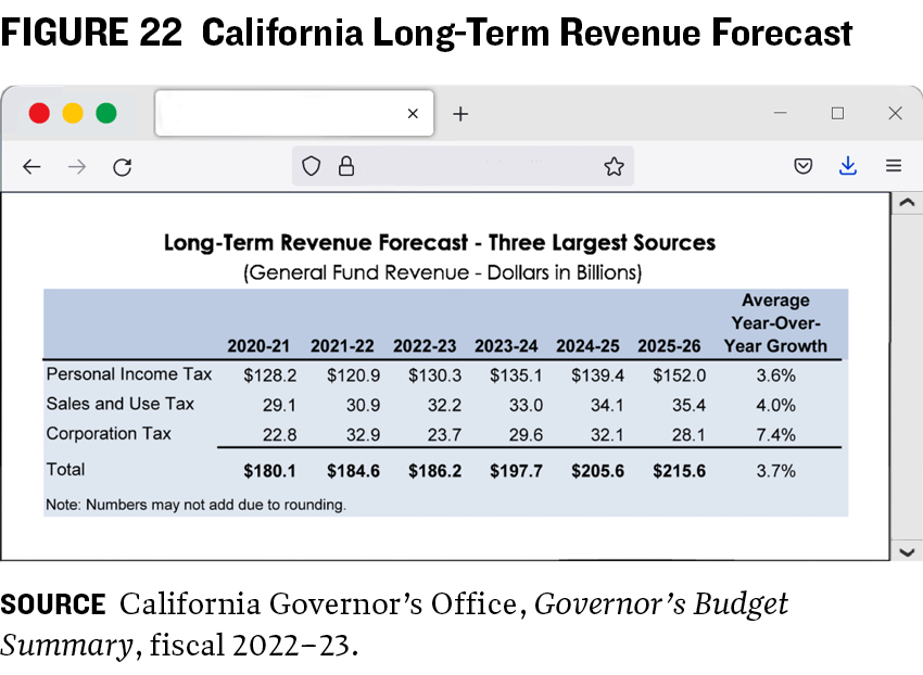
over the business cycle. However, the further projections are from the budget window, the more uncertain they become, driven more by shaky economic assumptions than by fundamental budget policy assumptions. In an interview, Connecticut executive budget officer Greg Messner, said that even though the state conducts longer-term forecasts, the single most important year outside the budget window is the first one because out-year forecasts become more speculative. Even with this high degree of uncertainty, a key benefit of forecasts beyond the budget window is to ensure that policymakers contemplate and incorporate best estimates of the long-term effects of their decisions.43
The following examples from Connecticut and California (figures 21 and 22) show how the states publicly convey longterm forecasts.
 Unlike a “hard” budget window forecast for an adopted budget that requires achieving balance, out-year forecasts generally represent “soft” estimates that do not require balancing. State officials take action to balance out-years in future budget cycles when they do fall within the budget window. This soft constraint on future budgets creates the potential for intentional fiscal manipulation, which could lead to fiscal shortfalls if legislation is enacted based on revenues that don’t materialize. Although requiring forecasts to incorporate the fiscal impacts of legislation beyond the budget window does not necessarily resolve that issue, it may make such questionable practices less attractive.
C. Beyond the Baseline Forecast
Each year, legislators propose budget policy changes through increases and decreases in spending and revenue. States often follow different processes for projecting the fiscal impacts of these policy changes than for the baseline forecasts of the effects on current policy. Depending on the state, these forecasts may involve executive or legislative budget staff.44
States often use different processes to forecast existing policy continuation and new policy creation. The budget process often begins by forecasting baseline revenues and spending for current policy, followed by different estimates for proposed and enacted budget changes. In this way, a current policy forecast often establishes the basic budget negotiation parameters for policy changes, including spending and tax policy changes over or below that baseline. Notably, current policy does not equal the specific dollar amounts in the prior year’s budget. Revenue estimates for current law will vary with changing economic conditions, as well as with previously enacted changes to tax policy. For example, as incomes grow, income tax revenues automatically increase without any new change to state tax law. An enacted tax rate cut will also adjust revenues going forward. A current-law baseline forecast adjusts for these changes.
States generally budget spending incrementally, with the starting point usually tied to the prior year’s budget. For example, states will generally back out one-time spending from the prior budget and may start at a fixed amount of (2 percent less, for example) than in that budget.
In addition, states may engage in autopilot budgeting, in which some new spending is built into the baseline up front rather than competing for priority. Examples include automatic spending adjustments for enrollment, caseload, or other changes in the number of people covered by certain large programs, such as education or Medicaid; inflation adjustments based on the consumer price index for specified items such as teachers’ contracts; or other modifications to the prior year’s budget. States that maintain more budget flexibility may add these items as distinct policy decisions in the budget prioritization process instead of automatically including them in a funding baseline. Many state budget challenges stem directly from the constraints that autopilot budgeting puts on budgetary flexibility.
New policy forecasts generally follow later in the process as governors and legislators review available revenues, then make recommendations and advance bills with new budget impacts through the legislative process. Legislative or executive branch staff may prepare fiscal estimates for new legislation. NASBO indicates that executive branch staffers in thirty-five states are involved to some extent in preparing fiscal notes on bills and that soley legislative staff perform that task in the other fifteen states.45
In some states, these bill estimates are public and formal, while in other states they are much less so. Unlike a baseline revenue estimate for the general fund, which often involves a team of forecasters, a new bill’s fiscal note may originate with a single analyst or much smaller group of people. Some of the greatest risks to state budgets come not from baseline revenue or spending forecasts but from policy changes whose fiscal impacts are not well understood. At least for major changes, these merit scrutiny on a level similar to baseline forecasts.
In addition, those seeking to get a bill passed may want to minimize the estimate of its fiscal impact. Depending on a state’s protocols for fiscal estimates, bill proponents may desire to delay or phase in implementation to shift the full cost of the measure beyond the traditional budget window. This pushes the true fiscal impact to a subsequent baseline forecast. To avoid such outcomes, states should disclose new legislation’s accurate fiscal cost by incorporating the ongoing budget impact of full implementation, no matter when a bill goes into effect. Even with solid baseline forecasting procedures, lack of a rigorous process to fully reflect long-term impacts of new spending or tax changes undermines sound fiscal management. Making changes without vetting fiscal assumptions can lead to significant problems, even if the baseline forecast is highly accurate.
D. Using Capital Budgeting to Manage the Process
Capital budgeting is by nature a long-term exercise. Major capital projects can involve debt service commitments that last for decades, similar to the asset’s long-term expected life. Capital budgeting can also be used to help manage the budget process over the business cycle.States that have dedicated ongoing revenues to one-time construction programs can delay or finance projects with bonds when a downturn hits. This would free up ongoing spending capacity for other purposes.
Failure to forecast the full capital costs of new buildings and roads also raises long-term structural imbalance concerns, as ongoing maintenance expenses are sometimes neglected. Unless a new building replaces another with similar maintenance costs, the expense of keeping up a new facility should be factored into the forecast, rather than dealing with a structural budget deficit years later when construction is completed.
4. The State Fiscal Tool Kit
Forecasting represents just one important instrument in the fiscal tool kit. State budget makers can employ a broad range of tools, or relief valves, to balance budgets. These tools are established, maintained, and constrained by state constitutions, statutes, executive orders, agency administrative rules, historical practice, and politics. Other critical state budget tools include:
- revenue system design, including the ability to raise or lower tax and fee levels and select revenue structures with more or less volatility;
- a range of budget reserves, including formal rainy day funds, unappropriated balances in general funds and an array of restricted accounts and working rainy day funds, or ongoing revenues allocated to one-time projects;
- cash flow management, including internal and external borrowing capacity and budget allocation timing; and
- the ability to control and adjust agency spending.
As described below, these budget tools can and should be incorporated into budget forecasting. For instance, the design of a state’s revenue structure is one important budget management tool. A state with highly volatile revenue may need to exercise more caution in forecasting to mitigate downside risk, while states with more reliable revenue may permit a less guarded forecast. Likewise, states can address their forecast uncertainty by designing their revenue system to have less volatile income streams.
A. The Structure of a State’s Economy Drives Forecasts, Revenues, and Budgets
Tax revenues and spending vary among states because of different taxing and spending policy choices and the interaction of those policies with fundamental state economic differences. Not surprisingly, budgets are closely tied to and often reflect state economies. The Hachman Index (figure 23) compares the composition of each state’s gross domestic product with that of the US. The index is based on the concept of a location quotient, the closer an index score is to 100, the more that state’s economy mirrors the nation’s economy (which is assumed to be broad and diverse).46
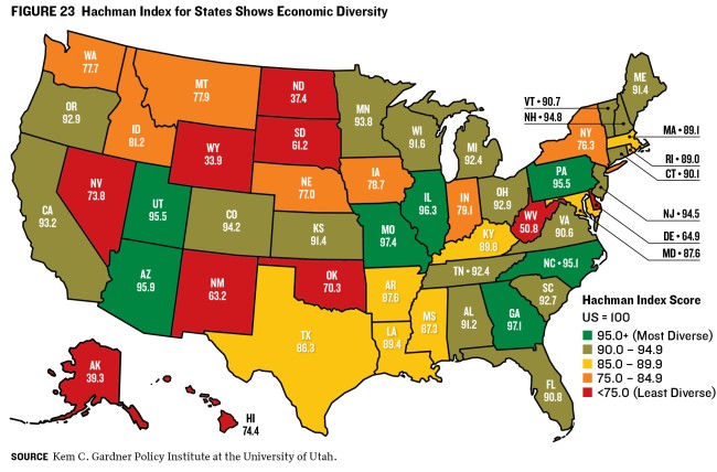
Although in some cases it may not be possible or desirable for a state to perfectly mirror the US economy, states with all their eggs in one economic basket can face budget management hurdles that require different approaches than those taken by states with more diverse economies.
For example, states such as Alaska, Wyoming, and North Dakota, which rely on natural resources for revenues, have some of the lowest Hachman Index scores. Their dependence on a volatile sector carries tremendous budget implications for these states. When oil and gas prices skyrocket, so do state revenues. When they plunge, revenues do likewise.
States with highly volatile and difficult-to-forecast revenue streams, such as those dependent on the personal income taxes of high earners (see California case study) or severance taxes on natural resources, must take a longer-term budgeting view; they may need to consider forecasting conservatively and reserving large amounts in good years to offset downturns, which are inevitable but difficult to forecast. For example, Alaska’s volatile general fund revenues require hefty reserves and a clear plan for replenishing them when oil prices spike. A state with more predictable revenue may not need reserves of such size.
Even given a similar economic structure, different choices about which taxes to impose and at what levels can change forecasting results. Some tax policy choices lead to more predictable outcomes than others. States with taxes that have less predictable outcomes should reflect that lack of predictability in their forecast, budget reserve, and other policies.
B. Understanding Revenue Volatility Is Key
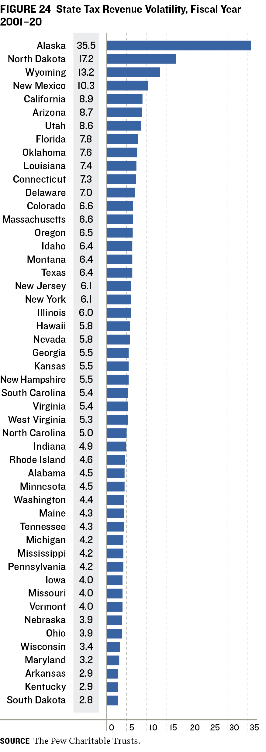 In examining state tax revenues collections, which reflect the effects of both economic and tax policy changes, professors Gary Cornia and Ray Nelson47 of Brigham Young University found in a report published by the Federal Reserve Bank of St. Louis that income taxes—particularly those levied on corporations—tend to be more volatile than general sales taxes, while property and motor fuel taxes are more stable. More volatile tax structures, such as those measured by the Pew Charitable Trusts’ volatility score (figure 24), create more forecasting difficulties.
Federal Reserve Bank of Chicago economists Rick Mattoon and Leslie McGranahan48 find increasingly volatile state revenues over time, largely due to increased reliance on income taxes. Similarly, Nathan Seegert,49 a University of Utah associate finance professor, finds that between 2000 and 2014, volatility in state tax revenues increased to 10.8 percent of tax receipts from 2.9 percent in the previous three decades. Seegert finds that 59 percent of the greater volatility comes from the states’ increased reliance on income taxes. Of the remaining volatility, increased economic swings explain about 22 percent, while other factors account for 19 percent.
These findings have important budget forecasting implications. One approach to mitigating the increased budget risk that volatility presents is to alter the revenue structure, generally by broadening the tax base to cover economic activity more comprehensively. Otherwise, states must figure out how to manage greater volatility with various budget tools, such as designing risk-averse forecasts and beefing up rainy day funds. Forecast approaches and tools that were adequate in prior eras may no longer meet state needs.
C. The Role of Fiscal Reserves
States have a broad range of budget reserves, including formal rainy day funds, unappropriated balances in the general fund, and restricted accounts. Some states also employ working rainy day funds in the form of ongoing revenues allocated to one-time projects. This approach builds a structural surplus and keeps tax revenues working in the state’s economy but provides budget flexibility.
Many budget outsiders focus on formal rainy day fund reserves because they are relatively
easy to identify and track over time, but budget insiders know that reserves are much broader than the official accounts. These informal reserves, in the form of agency restricted-account and carryover balances, can be compared to the nuts that squirrels hide for future use. Smart budget officials know where these nut stashes are and look to redirect these funds to free up general fund revenues when needed.
Figure 25 shows NASBO’s latest estimates of both formal rainy day funds and informal budget reserves. As illustrated, in recent years the often-forgotten informal reserves were about as large as the formal rainy day funds and amounted to at least half the amounts in official rainy day funds.
But formal and informal budget reserve funds have the limitation of being a one-time resource. So-called working rainy day funds are ongoing budget allocations matched with one-time expenses. In effect, these create a structural surplus that can be redirected to cover recurring expenditures during a downturn. Working rainy day funds carry this name because, unlike a formal rainy day fund, the funds do not sit idle in an account. Rather ongoing funds are strategically deployed to one-time capital projects and remain working to create economic benefit.
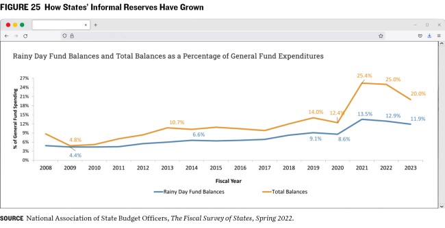
D. The Importance of Stress Testing
States should consider regular and formal scenario planning, stress testing their budget’s resiliency against economic downturns. Such exercises can provide officials with deeper insights into their fiscal preparedness. Like exercises required of banks since the Great Recession to test capital adequacy, budget stress testing evaluates a state’s preparation for a slump. Using several economic downturn scenarios, budget teams run the negative economic scenarios through their econometric models for major revenues and major spending categories. This produces a value at risk estimate that shows potential for revenue declines and spending increases on major programs such as Medicaid and education. Analysts then compare this estimate against a broad array of budget reserves to provide insight into the state’s fiscal preparation and to determine the extent to which additional budget buffers are needed.
E. Cash Flow Management
States have various tools to manage cash flow, including internal and external borrowing capacity and budget allocation timing. Many states carry large reserve funds, including rainy day funds, restricted account balances, and encumbered but unspent funds that remain in state accounts until contractors meet their contractual obligations. Subject to certain requirements, these accounts give states internal borrowing capacity to help manage cash flow.
Most states also maintain borrowing capacity, which allows them to tap financial markets when needed. This budget tool can ideally be paired with the working rainy day funds to manage the budget over the business cycle. This approach further benefits states because interest rates tend to drop during downturns, so at least a portion of a state’s borrowing occurs when money is comparatively cheap. However, a state that is already highly leveraged or confronting unfunded long-term liabilities may need to exercise greater caution in its overall budget approach, including forecasting.
In addition, states can control when appropriated funds are made available to state agencies. A prudent budget practice is to push budget increases into the budget year, rather than current year. If a downturn occurs before the beginning of the new fiscal year, as occurred for annual budget states during the pandemic, this spending can be fully or partially reversed before taking effect. States that adopt a budget close to the beginning of the budget year have less ability to employ this tool. States can also defer the timing of spending, delaying payments between fiscal years as a one-time tool, though the use of such cost-shifting maneuvers should be reserved for times of acute budget stress as they may be unsustainable in the long-term.
F. Agency Spending Levels and Controls
Most states can exercise strong control over agency spending. If projected revenues fail to materialize, many states provide automatic processes for midyear budget adjustments, such as directing the governor to make cuts. For budget-year allocations during a downturn, policymakers often have wide latitude to modify budgets. While dramatic cuts to some programs may create serious problems, a downturn often provides the political cover needed to challenge the assumption that every penny of government spending is worthwhile and merits preservation. Like a flash flood that clears out deadwood and refreshes life, budget challenges can allow policymakers to reprioritize state spending to critical and effective programs and to reexamine the state’s tax policies. Every budget director has a mental list of programs that are less valuable than others, but it is often challenging to adjust during good economic times. Although there may be legal, political, and practical constraints to cutting unneeded or less effective programs, all costs are variable in the long run.
Some states have large amounts of autopilot spending mandated by their constitutions, citizen initiatives, court settlements, or other contractual agreements such as employee collective bargaining deals. In addition, legacy costs for pensions and other long-term obligations should be incorporated when making forecasts. All else equal, limited budget flexibility should inform forecasting approaches to assume less risk.
CASE STUDY: California Has a Diverse Economy with Highly Volatile Revenue
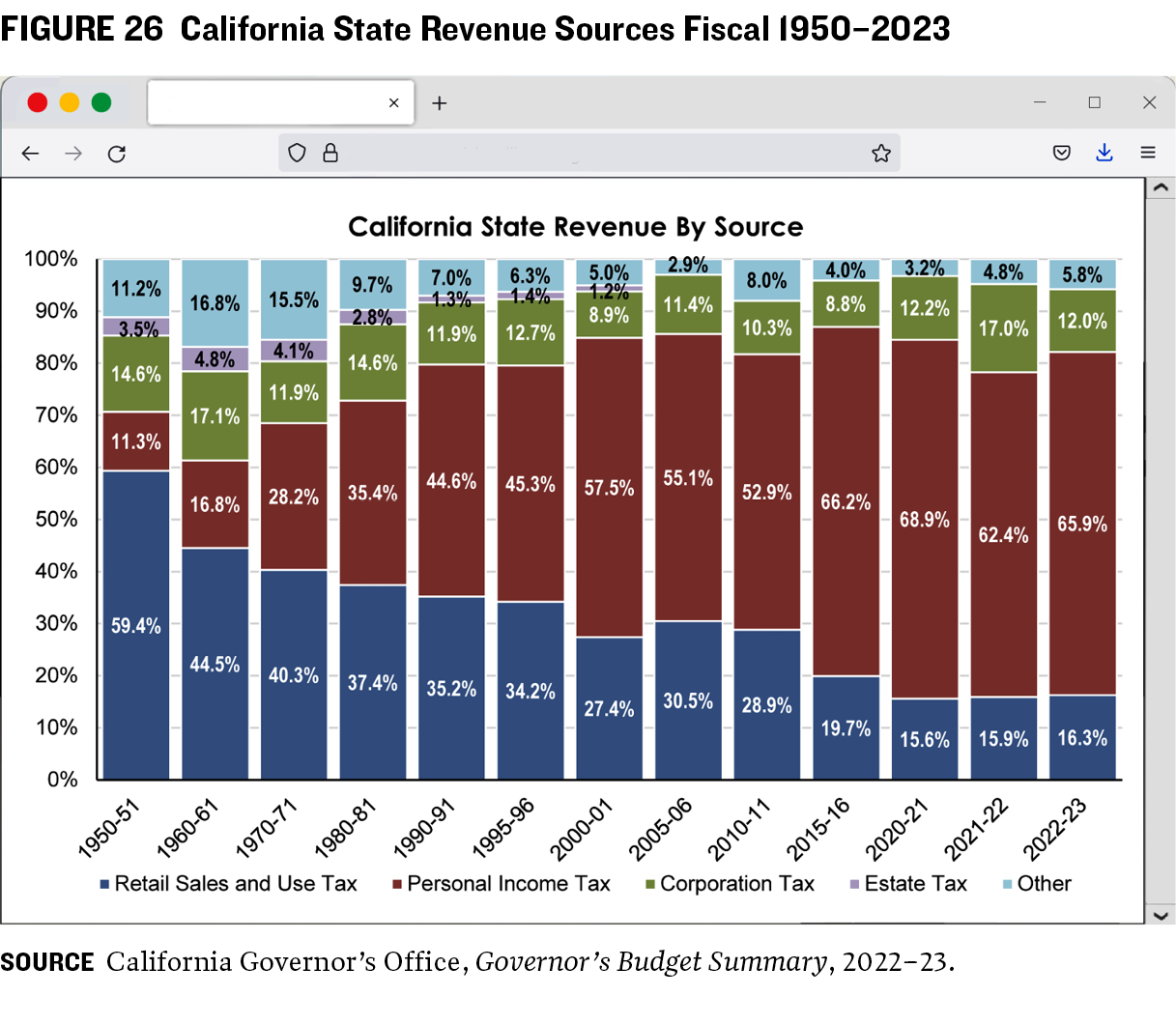 Unlike states that rely heavily on a single economic sector, California boasts significant economic diversity and tremendous economic advantages, including global trade access and impressive natural resources. Yet its less diverse tax portfolio subjects the state to revenue volatility that can create budget issues in downturns. Over the years, California made the policy decision to heavily tax some of the world’s biggest earners with a highly progressive income tax. During good years, this structure yields extraordinary revenue, as capital gains and business income skyrocket. Yet these incomes fluctuate tremendously, which creates major downside risk when the economy takes a turn for the worse.
As shown in figure 26, about 100,000 – or 0.5 percent – of California tax filers with over $1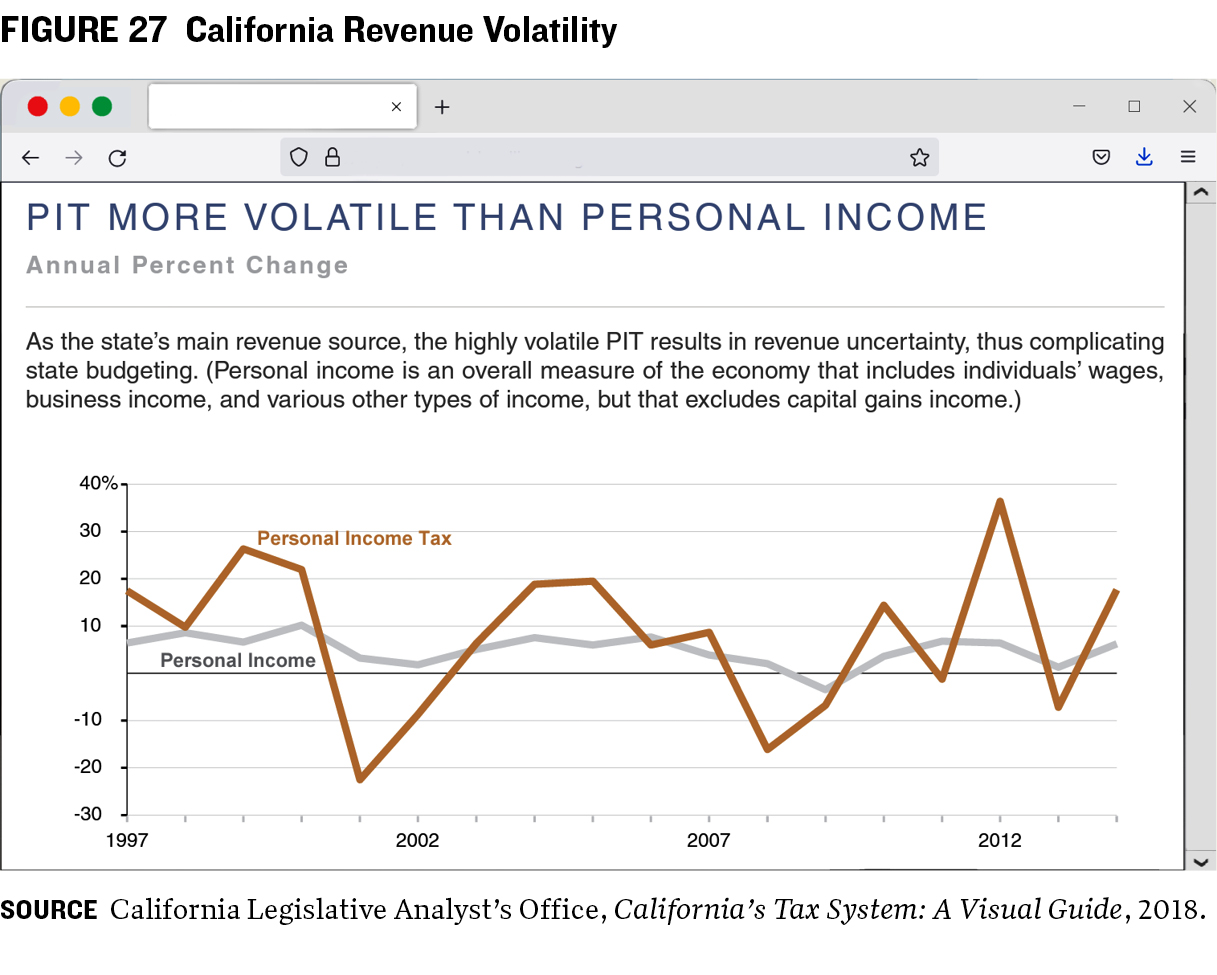 million in annual adjusted gross income pay about 40 percent of the state’s personal income taxes. This includes about 10,000 filers making over $5 million a year, who pay about 20 percent of income taxes.50 In large part due to the income variability of these top earners, the Legislative Analyst’s Office estimates that the state’s personal income tax is over five times as volatile as its total personal income (figure 27).51
CASE STUDY: Utah Budget Stress Testing
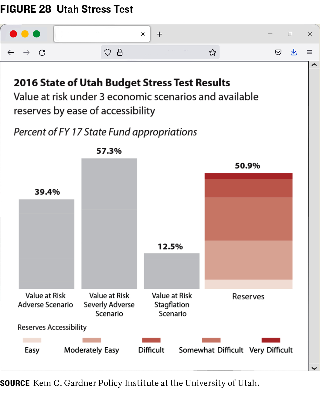 Fiscal preparations must occur before a crisis: It is too late to prepare for a storm when streets are already flooding. In Utah, where the author of this paper served as budget director from 2014–21, the state followed a fiscal sustainability playbook that had been developed over many years prior to the pandemic, particularly through an innovative budget stress-testing process (figure 28). Although the specific challenge of a pandemic had not been contemplated, officials had considered potential budget responses to a downturn of large magnitude. Rather than beginning to think through budget responses in the middle of a crisis, the state focused on execution and not last-second planning.
States should consider regular, formal scenario planning, or stress testing their budget’s resiliency against economic downturns and comparing budget reserves to value at risk measures.
ACKNOWLEDGMENTS
THIS REPORT WAS MADE POSSIBLE in part by a grant from the Peter G. Peterson Foundation. The statements made and views expressed are solely the responsibility of the author. We acknowledge the considerable support provided by the late Paul A. Volcker, the Volcker Alliance’s founding chairman, as well as the numerous academics, government officials, and public finance professionals who have guided the Alliance’s research on state budgets for the last seven years. We are also grateful for the invaluable guidance and direction of the many reviewers of this paper, which includes the staff of the National Association of State Budget Officers and the Utah Governor’s Office of Planning and Budget. Lastly, the report draws on Volcker Alliance special project consultants Katherine Barrett and Richard Greene's foundational work on the budget-forecasting process.
ENDNOTES
- Federal Reserve Bank of St. Louis, Continued Claims (Insured Unemployment), updated Sept. 15, 2022, link.
- Congressional Budget Office, Preliminary Estimate of the Effects of H.R. 748, the CARES Act, Public Law 116-136, Revised, With Corrections
to the Revenue Effect of the Employee Retention Credit and to the Modification of a Limitation on Losses for Taxpayers Other Than Corporations,
April 27, 2020, 1, link. - Board of Governors of the Federal Reserve System, Supervisory and Regulatory Actions in Response to COVID-19, August 2022, link.
- Phil Dean, “The Unprecedented Federal Fiscal Policy Response to the COVID-19 Pandemic and Its Impact on State Budgets,” California
Journal of Politics and Policy 14, no. 1 (2022), link. - US Bureau of Labor Statistics, Consumer Price Index for All Urban Consumers: All Items in US City Average, Sept. 13, 2022, link.
- National Association of State Budget Officers, Summary: Spring 2022 Fiscal Survey of States, June 16, 2022, 4, link.
- The Volcker Alliance, Truth and Integrity in State Budgeting: Preparing for the Storm, 2021, 9, link.
- The Volcker Alliance, Truth and Integrity in State Budgeting: Preparing for the Storm, 2021, 39, link.
- Gabriel Petek (California legislative analyst), interviews with research team, November 2021 – March 2022.
- Congressional Budget Office, “Troubled Asset Relief Program,” April 17, 2009, link.
- Congressional Budget Office, The Accuracy of CBO’s Budget Projections for Fiscal Year 2021, January 2021, 1–3, link.
- Congressional Budget Office, Report on the Troubled Asset Relief Program—July 2021, July 2021, 2, link.
- National Association of State Budget Officers, Summary: Fall 2020 Fiscal Survey of States, Dec. 23, 2020, 4, link.
- National Bureau of Economic Research, "US Business Cycle Expansions and Contractions,", link.
- US Bureau of Labor Statistics, Unemployment Rate, referenced Sept. 2, 2022, link.
- National Association of State Budget Officers, Summary: Fall 2020 Fiscal Survey of States, Dec. 23, 2020, 1, link.
- Phil Dean, "The Unprecedented Federal Fiscal Policy Response to the COVID-19 Pandemic and Its Impact on State Budgets", California Journal of
Politics and Policy 14, no. 1 (2022): 24, link. - Utah Office of the Legislative Fiscal Analyst, June 2020 Consensus Revenue, June 17, 2020, link.
- Congressional Budget Office, Preliminary Estimate of the Effects of H.R. 748, the CARES Act, Public Law 116–136, Revised, With Corrections
to the Revenue Effect of the Employee Retention Credit and to the Modification of a Limitation on Losses for Taxpayers Other Than Corporations,
April 27, 2020, 1, link. - The Volcker Alliance, Truth and Integrity in State Budgeting: Preparing for the Storm, 2021, 117, link.
- The Volcker Alliance, Truth and Integrity in State Budgeting: Preparing for the Storm, 2021, 53, link.
- Office of the Governor State of Idaho State Executive Department, Executive Order Number 2021-10, June 11, 2021, link.
- Alex Adams (administrator, Idaho Division of Financial Management), interviews with research team, November 2021 – March 2022.
- The Volcker Alliance, Truth and Integrity in State Budgeting: Preparing for the Storm, 2021, 43, link.
- The Volcker Alliance, Truth and Integrity in State Budgeting: Preparing for the Storm, 2021, 69, link.
- Keely Bosler (former director, California Department of Finance), interviews with research team, November 2021 – March 2022.
- Beverly S. Bunch, The $195 Billion Challenge: Facing State Fiscal Cliffs After COVID-19 Aid Expires, April 2022, 5, link.
- Marc Nicole (deputy secretary, Maryland Department of Budget and Management), interviews with research team, November 2021 – March 2022.
- The Volcker Alliance, Truth and Integrity in State Budgeting: Preparing for the Storm, 2021, 33, link.
- Alaska Permanent Fund Corporation, Invested with Alaskans: Fiscal Year 2022 Mid-Fiscal Year Review, Dec. 2021, 2, link.
- Alaska Department of Revenue, Spring 2022 Revenue Forecast, March 15, 2022, 13, link.
- Alaska Office of Management and Budget Officials, interviews with research team, November 2021 – March 2022.
- Alaska Department of Revenue, Revenue Sources Book: Fall 2021, Fall 2021, 8, link.
- Alaska Legislative Finance Division, The Fiscal Year 2023 Budget: Legislative Fiscal Analyst's Overview of the Governor's Request, January
2022, 5, link. - Donald J. Boyd and Lucy Dadayan, State Tax Revenue Forecasting Accuracy: Technical Report, September 2014, 39, link.
- Comptroller of Maryland, “Comptroller Provides Updated Revenue Forecast in Light of COVID-19,” news release, April 10, 2020, link.
- Comptroller of Maryland, Sales and Use Tax Comparative Statement of Net Receipts for the Year Ended June 2020 and 2019, 2020, link.
- National Association of State Budget Officers, Budget Processes in the States 2021, Spring 2021, 9, link.
- National Association of State Budget Officers, Budget Processes in the States 2021, Spring 2021, 30, link.
- Congressional Research Service, State Sales and Use Tax Nexus After South Dakota v. Wayfair, May 14, 2021, 1, link.
- National Association of State Budget Officers, Summary: Spring 2022 Fiscal Survey of States, June 16, 2022, 9, link.
- National Association of State Budget Officers, Summary: Spring 2022 Fiscal Survey of States, June 16, 2022, link.
- Greg Messner (executive budget officer, State of Connecticut Office of Policy and Management), interviews with research team, November 2021 – March 2022.
- National Association of State Budget Officers, Budget Processes in the States 2021, Spring 2021, 7, link.
- National Association of State Budget Officers, Budget Processes in the States 2021, Spring 2021, 21, link.
- Utah Economic Council, Economic Report to the Governor, 2022, 75, link.
- Gary C. Cornia and Ray D. Nelson, “State Tax Revenue Growth and Volatility,” Federal Reserve Bank of St. Louis Regional Economic
Development 6, no. 1 (2010): 41, link. - Rick Mattoon and Leslie McGranahan, State Tax Revenues over the Business Cycle: Patterns and Policy Responses, Chicago Fed Letter no.
299, June 2012, 3, link. - Nathan Seegert, Tax Revenue Volatility, June 3, 2016, 14, link.
- State of California Franchise Tax Board, PIT [Personal Income Tax] Annual Report 2020, Nov. 4, 2021, 4, link.
- California Legislative Analyst’s Office, California’s Tax System: A Visual Guide, April 12, 2018, 11, link.
© 2022 VOLCKER ALLIANCE INC.
Published November, 2022
The Volcker Alliance Inc. hereby grants a worldwide, royalty-free, non-sublicensable, non-exclusive license to download and distribute the Volcker Alliance paper titled A Cloudy Crystal Ball: Pandemic Forecasting Challenges Highlight Need for Various Budget Relief Valves (the “Paper”) for non-commercial purposes only, provided that the Paper’s copyright notice and this legend are included on all copies.
This paper was published by the Volcker Alliance as part of its Truth and Integrity in Government Finance Initiative. The views expressed in this paper are those of the authors and do not necessarily reflect the position of the Volcker Alliance. Any errors or omissions are the responsibility of the authors.
Don Besom, art director; Michele Arboit, copy editor; Stephen Kleege, editor.
